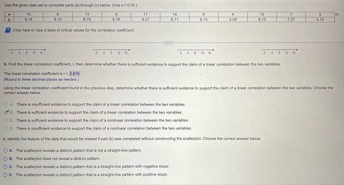
Use the given data set to complete parts (a) through (c) below. (Use α = 0.05.) X y 10 9.14 8 8.15 13 8.75 9 8.76 Click here to view a table of critical values for the correlation coefficient. 4 8 12 16 4 8 12 16 11 9.27 14 8.11 6 6.13 4 3.09 12 9.13 7 7.27 5 4.74 4 8 12 16 04 8 12 16 b. Find the linear correlation coefficient, r, then determine whether there is sufficient evidence to support the claim of a linear correlation between the two variables. The linear correlation coefficient is r = 0.816. (Round to three decimal places as needed.) Using the linear correlation coefficient found in the previous step, determine whether there is sufficient evidence to support the claim of a linear correlation between the two variables. Choose the correct answer below. OA. There is insufficient evidence to support the claim of a linear correlation between the two variables. B. There is sufficient evidence to support the claim of a linear correlation between the two variables. OC. There is sufficient evidence to support the claim of a nonlinear correlation between the two variables. OD. There is insufficient evidence to support the claim of a nonlinear correlation between the two variables. c. Identify the feature of the data that would be missed if part (b) was completed without constructing the scatterplot. Choose the correct answer below. OA. The scatterplot reveals a distinct pattern that is not a straight-line pattern. OB. The scatterplot does not reveal a distinct pattern. OC. The scatterplot reveals a distinct pattern that is a straight-line pattern with negative slope. OD. The scatterplot reveals a distinct pattern that is a straight-line pattern with positive slope. Table of Critical Values n a = .05 a = .01 4 .950 .990 5 .878 .959 6 .811 .917 7 .754 .875 8 .707 .834 9 .666 .798 10 .632 .765 11 .602 .735 12 .576 .708 13 .553 .684 14 .532 .661 15 .514 .641 16 .497 .623 17 .482 .606 18 .468 .590 19 .456 .575 20 .444 .561 25 .396 .505 30 .361 .463 35 .335 .430 40 .312 .402 45 .294 .378 50 .279 .361 60 .254 .330 70 236 .305 80 220 286 90 .207 .269 100 196 256 NOTE: To test Hop = 0 against H: p = 0, reject Ho if the absolute value of r is greater than the critical value in the table.

Use the given data set to complete parts (a) through (c) below. (Use a=0.05.) 10 13 11 14 8.84 12 y 7.45 6.77 12.73 7.11 7.81 6.08 5.39 8.16 6.41 5.72 Click here to view a table of critical values for the correlation coefficient. * KIR MM IVY E Using the linear correlation coefficient found in the previous step, determine whether there is sufficient evidence to support the claim of a linear correlation between the two variables. Choose the correct answer below. O A. There is sufficient evidence to support the claim of a nonlinear correlation between the two variables. O B. There is insufficient evidence to support the claim of a nonlinear correlation between the two variables. O C. There is sufficient evidence to support the claim of a linear correlation between the two variables. D. There is insufficient evidence to support the claim of a linear correlation between the two variables. c. Identify the feature of the data that would be missed if part (b) was completed without…

Use the given data set to complete parts (a) through (c) below. (Use a = 0.05.) 10 8 13 9. 11 14 4 12 7 y 7.45 6.77 12.73 7.11 7.81 8.84 6.08 5.39 8.16 6.41 5.72 Click here to view a table of critical values for the correlation coefficient. Using the linear correlation coefficient found in the previous step, determine whether there is sufficient evidence to support the claim of a linear correlation between the two variables. Choose the correct answer below. O A. There is sufficient evidence to support the claim of a nonlinear correlation between the two variables. O B. There is insufficient evidence to support the claim of a nonlinear correlation between the two variables. O C. There is sufficient evidence to support the claim of a linear correlation between the two variables. O D. There is insufficient evidence to support the claim of a linear correlation between the two variables. c. Identify the feature of the data that would be missed if part (b) was completed without constructing…

(Use alpha equals​0.05.) a. Construct a scatterplot.  b. Find the linear correlation​ coefficient, r, then determine whether there is sufficient evidence to support the claim of a linear correlation between the two variables. The linear correlation coefficient is r= ​(Round to three decimal places as​ needed.)

Use the given data set to complete parts​ (a).​ (Use α=​0.05.)   a. Find the linear correlation​ coefficient, r, then determine whether there is sufficient evidence to support the claim of a linear correlation between the two variables.   The linear correlation coefficient is r= ​(Round to three decimal places as​ needed.)

Use the given data set to complete parts​ (a) through​ (c) below.​ (Use α=​0.05.)   x 10 8 13 9 11 14 6 4 12 7 5   y 9.14 8.14 8.74 8.78 9.26 8.11 6.12 3.11 9.12 7.26 4.73       LOADING... Click here to view a table of critical values for the correlation coefficient.       a. Construct a scatterplot. Choose the correct graph below.     A.       04812160246810xy         A scatterplot has a horizontal x-scale from 0 to 16 in increments of 2 and a vertical y-scale from 0 to 10 in increments of 1. Eleven points strictly follow the pattern of a line passing through the points (4, 6) and (14, 1). All coordinates are approximate.   B.       04812160246810xy         A scatterplot has a horizontal x-scale from 0 to 16 in increments of 2 and a vertical y-scale from 0 to 10 in increments of 1. Eleven points strictly follow the pattern of a curve that rises from left to right passing through the…

Annual high temperatures in a certain location have been tracked for several years. Let XX represent the year and YY the high temperature. Based on the data shown below, calculate the correlation coefficient (to three decimal places) between XX and YY. Use your calculator! x y 3 14.3 4 13.89 5 15.58 6 14.87 7 12.66 8 10.15 9 9.54 10 8.13 11 11.42 12 9.81 13 6.6 r=

Use the given data set to complete parts (a) through (c) below. (Use a = 0.05.) 10 8 13 11 14 6 4 12 7 5 y 7.46 6.77 12.74 7.11 7.81 8.84 6.09 5.39 8.14 6.43 5.72 Click here to view a table of critical values for the correlation coefficient. A. В. O C. D. Ay 16- Ay 16- Q Ay 16- Ay 16- Q 12- 12- 12- 12- 8- 8- 8- 8- .. 4- 4- 4- 4- 0- 4 0- 0- 0+ 4 12 16 4 12 16 16 4 12 16 b. Find the linear correlation coefficient, r, then determine whether there is sufficient evidence to support the claim of a linear correlation between the two variables. The linear correlation coefficient is r= 0.816. (Round to three decimal places as needed.) Using the linear correlation coefficient found in the previous step, determine whether there is sufficient evidence to support the claim of a linear correlation between the two variables. Choose the correct answer below. A. There is insufficient evidence to support the claim of a nonlinear correlation between the two variables. B. There is sufficient evidence to…

Use the given data set to complete parts (a) through (c) below. (Use a = 0.05.) х 10 8 13 11 14 4 12 У 9.14 8.14 8.74 8.77 9.25 8.09 6.14 3.11 9.13 7.26 4.74 Click here to view a table of critical values for the correlation coefficient. a. Construct a scatterplot. Choose the correct graph below. ici O A. B. OC. OD. Ay 10- Ay 10- Ay 10- Ay 10- 8- 8- 8- 8- 6- 6- 6- 6- 4- 4- 4- 4- 2- 2- 2- 2- 0- 0+ 0+ 4 0+ 4 12 16 8 12 16 12 16 4 12 16 b. Find the linear correlation coefficient, r, then determine whether there is sufficient evidence to support the claim of a linear correlation between the two variables. The linear correlation coefficient is r= (Round to three decimal places as needed.) Using the linear correlation coefficient found in the previous step, determine whether there is sufficient evidence to support the claim of a linear correlation between the two variables. Choose the correct answer below. A. There is insufficient evidence to support the claim of a linear correlation between…

Use the given data set to complete parts (a) through (c) below. (Use a =0.05.) 10 8 13 9. 11 14 4 12 7 y 9.15 8.14 8.74 8.77 9.25 8.11 6.12 3.09 9.14 7.26 4.74 Click here to view a table of critical values for the correlation coefficient. Ay 10- Ay 10- 本Y 10- y 10- 8- 8- 6- 8- 8- 6- 6- 6- 4- 4- 4 4. 2- 2- 2- 2- 0- 4 8 12 16 4 8 12 16 4 18 12 16 4 8. 12 16 b. Find the linear correlation coefficient, r, then determine whether there is sufficient evidence to support the claim of a linear correlation between the two variables. The linear correlation coefficient is r= (Round to three decimal places as needed.)