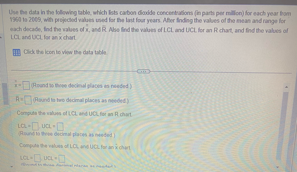
Use the data in the following table, which lists carbon dioxide concentrations (in parts per million) for each year from 1960 to 2009, with projected values used for the last four years. After finding the values of the mean and range for each decade, find the values of x, and R. Also find the values of LCL and UCL for an R chart, and find the values of LCL and UCL for an x chart. Click the icon to view the data table. (Round to three decimal places as needed.) (Round to two decimal places as needed.) Compute the values of LCL and UCL for an R chart. LCL= L=,UCL = (Round to three decimal places as needed.) Compute the values of LCL and UCL for an x chart. X= R= LCL= UCL = (Round to three decimal nlaras ac noorled)

Data: 3.5, 3.2, 3.1, 3.5, 3.6, 3.2, 3.4, 2.9, 4.1, 2.6, 3.3, 3.5, 3.9, 3.8, 3.7, 3.4, 3.6, 3.5, 3.5, 3.7, 3.6, 3.8, 3.2, 3.4, 4.2, 3.6, 3.1, 2.9, 2.5, 3.5, 3.1, 3.2, 3.7, 3.8, 3.4, 3.6, 3.5, 3.2, 3.6, 3.8 Sketch a histogram with ranges of 0.1, from minimum (2.5) to maximum (4.2) values. Then sketch a histogram with ranges of 0.3. You can include the relative frequency scales on the same sketches.

The pathogen Phytophthora capsici causes bell peppers to wilt and die. Because belI peppers are an important commercial crop, this disease has undergone a great deal of agricultural research. It is thought that too much water aids the spread of the pathogen. Two fields are under study. The first step in the research project is to compare the mean soil water content for the two fields. Units are percentage of water by volume of soil. Field A samples, x: 10.0 10.7 15.5 10.4 9.9 10.0 16.6 15.1 15.2 13.8 14.1 11.4 11.5 11.0 Field B samples, x,: 8.3 8.5 8.4 7.3 8.0 7.1 13.9 12.2 13.4 11.3 12.6 12.6 12.7 12.4 11.3 12.5 A USE SALT Use a calculator to calculate x,, s,,x,, and s,. (Round your answers to four decimal places.) x, (a) Assuming the distribution of soil water content in each field is mound-shaped and symmetric, use a 5% level of significance to test the claim that field A has, on average, a higher soil water content than field B. (1) What is the level of significance?

Suppose you are told your BMI is 32, the  70th percentile for your age and sex. Please interpret this percentile age: 28 Female

For each type of chart determine the type of variable that should be used

please answer 8d, e, and f.