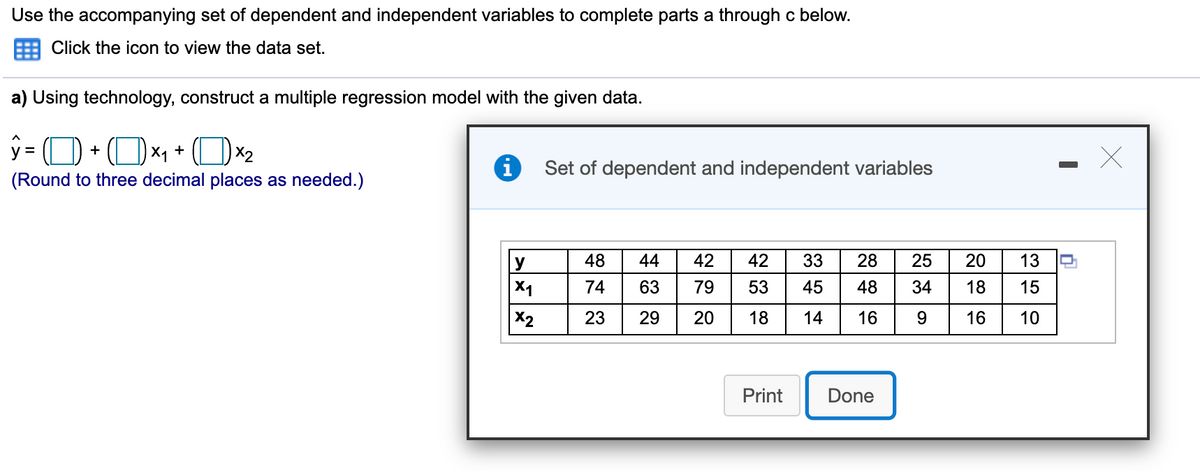
Use the accompanying set of dependent and independent variables to complete parts a through c below. Click the icon to view the data set. a) Using technology, construct a multiple regression model with the given data. X1 + X2 Set of dependent and independent variables (Round to three decimal places as needed.) y X1 48 44 42 42 33 28 25 20 13 74 63 79 53 45 48 34 18 15 X2 23 29 20 18 14 16 9 16 10 Print Done

The data show the chest size and weight of several bears. Find the regression equation, letting chest size be the independent (x) variable. Then find the best predicted weight of a bear with a chest size of 40 inches. Is the result close to the actual weight of 352 pounds? Use a significance level of 0.05. Chest size (inches) *Weight (pounds) 44 54 328 528 41 55 39 51 418 580 296 503 Click the icon to view the critical values of the Pearson correlation coefficient r. - What is the regression equation? x (Round to one decimal place as needed.)

Find the equation of the regression line for the given data. Then construct a scatter plot of the data and draw the regression line. (The pair of variables have a significant correlation.) Then use the regression equation to predict the value of y for each of the given x-values, if meaningful. The table below shows the heights (in feet) and the number of stories of six notable buildings in a city. Height, x Stories, y A 60- 0 775 53 Q 619 47 519 46 OB. 508 42 Find the regression equation. y = x+ (Round the slope to three decimal places as needed. Round the y-intercept to two decimal places as needed.) Choose the correct graph below. Q. A. 60 0 491 37 800 800 Height (feet) (n) Brodict the value of x for x=503. Choose the correct answer below. Height (feet) 474 36 D ... (a) x = 503 feet (c) x 310 feet OC. 800 0 Height (feet) Q www. (b)x=642 feet (d) x = 730 feet OD. 60- 0- 0 800 Height (feet)

Find the equation of the regression line for the given data. Then construct a scatter plot of the data and draw the regression line. (The pair of variables have a significant correlation.) Then use the regression equation to predict the value of y for each of the given x-values, if meaningful. The table below shows the heights (in feet) and the number of stories of six notable buildings in a city. Height, x Stories, y 762 51 621 46 515 45 508 42 491 39 480 36 (a) x = 502 feet (c) x = 315 feet Find the regression equation. ŷ=x+ (Round the slope to three decimal places as needed. Round the y-intercept to two decimal places as needed.) (b) x = 645 feet (d) x = 731 feet

In order for applicants to work for the foreign-service department, they must take a test in the language of the country where they plan to work. The data below shows the relationship between the number of years that applicants have studied a particular language and the grades they received on the proficiency exam. Find the equation of the regression line for the given data. Number of years, x 4 4 3 6 2 7 3 Grades on test, y 61 68 75 82 73 90 58 93 72 滷 O A. =6.910x+46.261 O B. y = 46.261x+6.910 OC. v=6.910x-46.261 OD. O D. y = 46.261x -6.910 Fi St 5e Assig

An instructor asked a random sample of eight students to record their study times at the beginning of a course. She then made a table for total hours studied​ (x) over 2 weeks and test score​ (y) at the end of the 2 weeks. The table is given below. Complete parts​ (a) through​ (f).   x 10 13 10 18 6 15 16 21   y 93 79 81 74 85 81 85 80   a. Find the regression equation for the data points. b. Graph the regresson equation c. Describe the apparent relationship between the two variables. d. Identify the predictor and response variables. e. Identify outliers and potential influential observations. f.Predict the score for a student that studies for 17 hours.

Use the data in the table below to complete parts​ (a) through​ (d).   x 37 34 40 46 42 50 62 56 51   y 22 20 25 32 27 30 30 25 28   Find the equation of the regression line.   y=

Roller coasters get their speed as a result of dropping down a steep incline. The table below gives height of a drop and the speed achieved for different roller coasters around the world. Drop in Meters (m        25      30       28        58      55      40      90      100 Speed of the coaster (k.p.h)           80           90             78            93          90         93        105       128   Have your calculator find the linear regression for the roller coaster data above. Write the linear model, clearly define the variables and state correlation coefficient and clearly interpret the slope.                   Use the model to find the drop height that will result in a coaster speed of 150 kph.     Have your calculator find the exponential regression for this data. Write the exponential model, clearly define the variables and state correlation coefficient.       Use the model to find the drop height that will result in a…

Find the equation of the regression line for the given data. Then construct a scatter plot of the data and draw the regression line. (The pair of variables have a significant correlation.) Then use the regression equation to predict the value of y for each of the given x-values, if meaningful. The table below shows the heights (in feet) and the number of stories of six notable buildings in a city. Height, x Stories, y 758 621 518 510 492 | 483 | 51 47 46 43 39 36 Find the regression equation. y = ☐ X+ (a) x = 503 feet (c) x = 802 feet (b) x = 649 feet (d) x = 728 feet (Round the slope to three decimal places as needed. Round the y-intercept to two decimal places as needed.)

Find the equation of the regression line for the given data. Then construct a scatter plot of the data and draw the regression line. (The pair of variables have a significant correlation.) Then use the regression equation to predict the value of y for each of the given x-values, if meaningful. The table below shows the heights (in feet) and the number of stories of six notable buildings in a city. 483 Height, x Stories, y 772 628 518 508 51 48 45 42 496 37 (a) x=499 feet (c) x=315 feet (b)x=639 feet (d) x = 732 feet 35 Find the regression equation. ŷ=x+ (Round the slope to three decimal places as needed. Round the y-intercept to two decimal places as needed.) Choose the correct graph below. O C. OB. O D. OA. Q Q ↓ 0 0 Height (feet) Height (feet) (a) Predict the value of y for x = 499. Choose the correct answer below. OA. 51 OB. 40 60+ 0- 800 60+ 0- 800 Q A 60- → 0 Height (feet) 800 60- 0- 800 0 Height (feet)