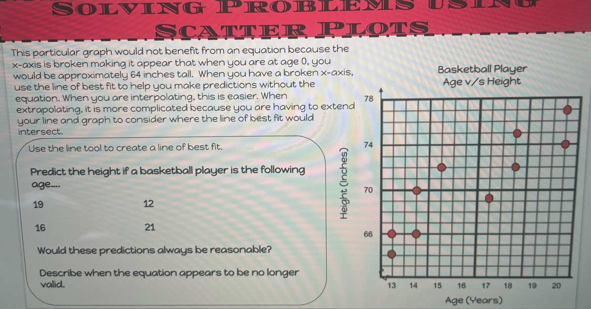
This particular graph would not benetit from an equat x-axis is broken making it appear that when you are at age 0, you would be approximately 64 inches tall. When you have a broken x-axis, use the line of best fit to help you make predictions without the equation. When you are interpolating, this is easier. When extrapolating, it is more complicated because you are having to extend your line and graph to consider where the line of best fit would intersect. Basketball Player Age v/s Height 78 74 Use the line tool to create a line of best fit. Predict the height if a basketball player is the following age. 70 19 12 16 21 66 Would these predictions always be reasonable? Describe when the equation appears to be no longer valid. 13 14 15 16 17 18 19 20 Age (Years) Height (Inches)

Range of ankle motion is a contributing factor to falls among the elderly. Suppose a team of researchers is studying how compression hosiery, typical shoes, and medical shoes affect range of ankle motion. In particular, note the variables Barefoot and Footwear2. Barefoot represents a subject's range of ankle motion (in degrees) while barefoot, and Footwear2 represents their range of ankle motion (in degrees) while wearing medical shoes. Use this data and your preferred software to calculate the equation of the least-squares linear regression line to predict a subject's range of ankle motion while wearing medical shoes, ?̂ , based on their range of ankle motion while barefoot, ? . Round your coefficients to two decimal places of precision. ?̂  = A physical therapist determines that her patient Jan has a range of ankle motion of 7.26°7.26° while barefoot. Predict Jan's range of ankle motion while wearing medical shoes, ?̂ . Round your answer to two decimal places. ?̂ = Suppose Jan's…

The scatter plot shows the time spent watching TV, x, and the time spent doing homework, y, by each of 23 students last week. (a) Write an approximate equation of the line of best fit for the data. It doesn't have to be the exact line of best fit. (b) Using your equation from part (a), predict the time spent doing homework for a student who spends 15 hours watching TV. Note that you can use the graphing tools to help you approximate the line. Time spent doing homework (in hours) 32 28 24 20 16+ 12 8 4 0 y XX 4 X X X X X X X X 8 12 X X 16 X X X X -X X 20 24 Time spent watching TV (in hours) X X X 28 32 X X Ś (a) Write an approximate equation of the line of best fit. y = 0 (b) Using your equation from part (a), predict the time spent doing homework for a student who spends 15 hours watching TV. hours X S

The scatter plot shows the time spent watching TV, x, and the time spent doing homework, y, by each of 23 students last week. (a) Write an approximate equation of the line of best fit for the data. It doesn't have to be the exact line of best fit. (b) Using your equation from part (a), predict the time spent doing homework for a student who spends 15 hours watching TV. Note that you can use the graphing tools to help you approximate the line. Time spent doing homework Kin hours) 32- 28- Y 244 20- 124 F 44 B * K 12 x 14 20 24 26 Time spent watching TV (in hours) 32 X (a) Write an approximate equation of the line of best fit. = 0 (b) Using your equation from part (a), predict the time spent doing homework for a student who spends 15 hours watching TV. hours