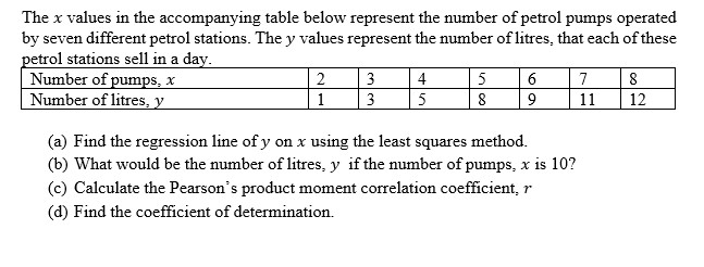
The x values in the accompanying table below represent the number of petrol pumps operated by seven different petrol stations. The y values represent the number of litres, that each of these petrol stations sell in a day. Number of pumps, x Number of litres, y 2 3 4 5 7 1 3 5 8 11 12 (a) Find the regression line of y on x using the least squares method. (b) What would be the number of litres, y if the number of pumps, x is 10? (c) Calculate the Pearson's product moment correlation coefficient, r (d) Find the coefficient of determination.

Suppose that the line ŷ = 5+ 2x is fitted to the data points (-2,2), (1,6), and (5,14). Determine the sum of the squared residuals. %3D Sum of the Squared Residuals =

A company that manufactures computer chips wants to use a multiple regression model to study the effect that 3 different variables have on y, the total daily production cost (in thousands of dollars). Let B,, B,, and B, denote the coefficients of the 3 variables in this model. Using 22 observations on each of the variables, the software program used to find the estimated regression model reports that the total sum of squares (SST) is 485.84 and the regression sum of squares (SSR) is 229.91. Using a significance level of 0.10, can you conclude that at least one of the independent variables in the model provides useful (i.e., statistically significant) information for predicting daily production costs? Perform a one-tailed test. Then complete the parts below. Carry your intermediate computations to three or more decimal places. (a) State the null hypothesis H, for the test. Note that the alternative hypothesis H, is given. H, :0 H, : at least one of the independent variables is useful…

For major league baseball teams, do higher player payrolls mean more gate money? Here are data for each of the National League teams in the year 2002. The variable x denotes the player payroll (in millions of dollars) for the year 2002, and the variable y denotes the mean attendance (in thousands of fans) for the 81 home games that year. The data are plotted in the scatter plot below, as is the least-squares regression line. The equation for this line is y =5.91+0.34x. Player payroll, x (in $1,000,000s) thousands) Мean attendance, y (in Arizona 103.5 39.51 Atlanta 93.8 32.10 45- Chicago Cubs 75.0 33.21 40- Cincinnati 46.3 22.96 35 Colorado 56.6 33.83 30- Florida 40.8 10.00 Houston 65.4 31.11 Los Angeles 101.5 38.64 15 Milwaukee 49.3 24.32 10- Montreal 37.9 10.00 New York Mets 94.4 34.57 120 140 Philadelphia 59.6 20.00 Player payroll, x (in $1,000,000s) Pittsburgh 46.1 21.98 San Diego 41.8 27.41 San Francisco 78.4 40.12 St Louis 76.2 37.16 Send data to calculator Send data to Excel…

For major league baseball teams, do higher player payrolls mean more gate money? Here are data for each of the National League teams in the year  2002 . The variable  x  denotes the player payroll (in millions of dollars) for the year  2002 , and the variable  y  denotes the mean attendance (in thousands of fans) for the  81  home games that year. The data are plotted in Figure 1 scatter plot, as is the least-squares regression line. The equation for this line is  =y+5.910.34x   . Answer the following:   1. Fill in the blank: For these data, mean attendance values that are less than the mean of the mean attendance values tend to be paired with player payroll values that are _____ the mean of the player payroll values. Choose onegreater thanless than 2. Fill in the blank: According to the regression equation, for an increase of one million dollars in player payroll, there is a corresponding _____ of 0.34 thousand fans in mean attendance. Choose…

An article gave a scatter plot, along with the least squares line, of x = rainfall volume (m³) and y data on rainfall and runoff volume (n = runoff volume (m³) for a particular location. The simple linear regression model provides a very good fit to 15) given below. The equation of the least squares line is y = -2.364 + 0.84267x, ² 0.976, and s = 5.21. = x 5 12 14 17 23 30 40 47 55 67 72 81 96 112 127 y 3 9 12 14 14 24 27 45 38 46 52 71 81 100 101 (a) Use the fact that s = 1.43 when rainfall volume is 40 m³ to predict runoff in a way that conveys information about reliability and precision. (Calculate a 95% PI. Round your answers to two decimal places.) Ŷ 28.25 1x ) m³ Does the resulting interval suggest that precise information about the value of runoff for this future observation is available? Explain your reasoning. OYes, precise information is available because the resulting interval is very wide. 34.46 Yes, precise information is available because the resulting interval is very…

Use the least squares regression line of this data set to predict a value. Meteorologists in a seaside town wanted to understand how their annual rainfall is affected by the temperature of coastal waters. For the past few years, they monitored the average temperature of coastal waters (in Celsius), x, as well as the annual rainfall (in millimetres), y. Rainfall statistics • The mean of the x-values is 11.503. • The mean of the y-values is 366.637. • The sample standard deviation of the x-values is 4.900. • The sample standard deviation of the y-values is 44.387. • The correlation coefficient of the data set is 0.896. The least squares regression line of this data set is: y = 8.116x + 273.273 How much rainfall does this line predict in a year if the average temperature of coastal waters is 15 degrees Celsius? Round your answer to the nearest integer. millimetres

For major league baseball teams, do higher player payrolls mean more gate money? Here are data for each of the American League teams in the year 2002. The variable x denotes the player payroll (in millions of dollars) for the year 2002, and the variable y denotes the mean attendance (in thousands of fans) for the 81 home games that year. The data are plotted in the scatter plot below, as is the least-squares regression line. The equation for this line is y = 11.43 + 0.23x. Player payroll, x (in Mean attendance, y (in $1,000,000s) thousands) Anaheim 62.8 28.52 Baltimore 56.5 33.09 40- Boston 110.2 32.72 35 Chicago White Sox 54.5 20.74 30- Cleveland 74.9 32.35 25- Detroit 54.4 18.52 Kansas City 49.4 16.30 15- Minnesota 41.3 23.70 10+ New York Yankees 133.4 42.84 Oakland 41.9 26.79 20 40 60 80 100 120 140 Seattle 86.1 43.70 Player payroll, Тarmpa Bay 34.7 13.21 X (in $1,000,000s) Техas 106.9 29.01 Toronto 66.8 20.25 Send data to calculator Send data to Excel Based on the sample data and…

To monitor and improve its productivity, a company made an investigation and found out that the factor that affects the productivity the most is the absenteeism. The company data analytics department have collected data about the two variables (Productivity and Absenteeism) for the 12 past years as shown in the table below. Now the purpose of the company is to determine, through regression analysis, whether the productivity is statistically affected by the absenteeism level or not. Year Absenteeism Productivity (in number of absent worker) (in Million AED) 1 204 342 2 352 336 3 154 406 4 206 410 5 422 278 6 530 214 7 750 138 8 482 268 9 374 262 10 120 356 11 188 396 12 634 152 Questions: Construct a scatter diagram for the data about productivity and absenteeism then interpret the possible relationship that can be found. Construct a simple regression model to predict the…

An engineer wants to determine how the weight of a​ gas-powered car,​ x, affects gas​ mileage, y. The accompanying data represent the weights of various domestic cars and their miles per gallon in the city for the most recent model year. Complete parts​ (a) through​ (d) below.   ​(a) Find the​ least-squares regression line treating weight as the explanatory variable and miles per gallon as the response variable.   y=nothingx+​(nothing​) ​(Round the x coefficient to five decimal places as needed. Round the constant to one decimal place as​ needed.) ​(b) Interpret the slope and​ y-intercept, if appropriate. Choose the correct answer below and fill in any answer boxes in your choice. ​(Use the answer from part a to find this​ answer.)   A. A weightless car will get nothing miles per​ gallon, on average. It is not appropriate to interpret the slope.   B. For every pound added to the weight of the​ car, gas mileage in the city will decrease by nothing ​mile(s) per​ gallon, on…