The following three independent random samples are obtained from three normally distributed populations with equal variance. The dependent variable is starting hourly wage, and the groups are the types of position (internship, co-op, work study). We are testing the claim that the starting salaries for new college graduate are different depending on the positions at α=0.05α=0.05 given the following dataGroup 1: InternshipGroup 2: Co-opGroup 3: Work Study14131515.25101212.25119.51312.5121312.59131012.7514.251211.512.2511.511.7511.2513.7511.7514.51513.5 Your friend Adrianna helped you with the null and alternative hypotheses...H0: μ1=μ2=μ3H0: μ1=μ2=μ3H1:H1: At least one of the mean is different from the others.The test-statistic for this data = (Please show your answer to 3 decimal places.) The p-value for this sample = (Please show your answer to 4 decimal places.)

Name: The following three independent random samples are obtained from three
Uploaded: 2024-03-20T07:07:12.000Z
Channel: Bartleby
Description: The following three independent random samples are obtained from three normally distributed populations with equal variance. The dependent variable is starting hourly wage, and the groups are the types of position (internship, co-op, work study). We

Answered: The test-statistic for this data =…

MATLAB: An Introduction with Applications

6th Edition

ISBN:9781119256830

Author:Amos Gilat

Publisher:Amos Gilat

Chapter1: Starting With Matlab

Section: Chapter Questions

Problem 1P

See similar textbooks

Related questions

Topic Video

Question

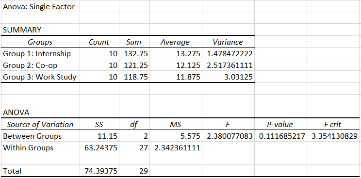
The following three independent random samples are obtained from three normally distributed populations with equal variance. The dependent variable is starting hourly wage, and the groups are the types of position (internship, co-op, work study). We are testing the claim that the starting salaries for new college graduate are different depending on the positions at α=0.05α=0.05 given the following data

Group 1: Internship	Group 2: Co-op	Group 3: Work Study
14	13	15
15.25	10	12
12.25	11	9.5
13	12.5	12
13	12.5	9
13	10	12.75
14.25	12	11.5
12.25	11.5	11.75
11.25	13.75	11.75
14.5	15	13.5

Your friend Adrianna helped you with the null and alternative hypotheses...
H0: μ1=μ2=μ3H0: μ1=μ2=μ3
H1:H1: At least one of the mean is different from the others.
The test-statistic for this data = (Please show your answer to 3 decimal places.)

The p-value for this sample = (Please show your answer to 4 decimal places.)

Features Features Normal distribution is characterized by two parameters, mean (µ) and standard deviation (σ). When graphed, the mean represents the center of the bell curve and the graph is perfectly symmetric about the center. The mean, median, and mode are all equal for a normal distribution. The standard deviation measures the data's spread from the center. The higher the standard deviation, the more the data is spread out and the flatter the bell curve looks. Variance is another commonly used measure of the spread of the distribution and is equal to the square of the standard deviation.

Expert Solution

Working

We have used the excel data analysis tool to run the ANOVA analysis.

Trending now

This is a popular solution!

Step by step

Solved in 2 steps with 1 images

SEE SOLUTION Check out a sample Q&A here

Knowledge Booster

$Hypothesis Tests and Confidence Intervals for Means$

Learn more about

Need a deep-dive on the concept behind this application? Look no further. Learn more about this topic, statistics and related others by exploring similar questions and additional content below.

Similar questions