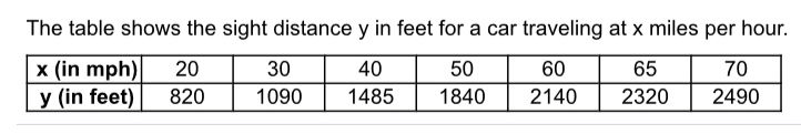
The table shows the sight distance y in feet for a car traveling at x miles per hour. x (in mph) y (in feet) 20 30 40 50 60 65 70 1090 820 1485 1840 2140 2320 2490

The scatter plot shows the time spent watching TV, x, and the time spent doing homework, y, by each of 23 students last week. (a) Write an approximate equation of the line of best fit for the data. It doesn't have to be the exact line of best fit. (b) Using your equation from part (a), predict the time spent doing homework for a student who spends 15 hours watching TV. Note that you can use the graphing tools to help you approximate the line. Time spent doing homework (in hours) 32 28 24 20 16+ 12 8 4 0 y XX 4 X X X X X X X X 8 12 X X 16 X X X X -X X 20 24 Time spent watching TV (in hours) X X X 28 32 X X Ś (a) Write an approximate equation of the line of best fit. y = 0 (b) Using your equation from part (a), predict the time spent doing homework for a student who spends 15 hours watching TV. hours X S

The scatter plot shows the time spent watching TV, x, and the time spent doing homework, y, by each of 23 students last week. (a) Write an approximate equation of the line of best fit for the data. It doesn't have to be the exact line of best fit. (b) Using your equation from part (a), predict the time spent doing homework for a student who spends 15 hours watching TV. Note that you can use the graphing tools to help you approximate the line. Time spent doing homework Kin hours) 32- 28- Y 244 20- 124 F 44 B * K 12 x 14 20 24 26 Time spent watching TV (in hours) 32 X (a) Write an approximate equation of the line of best fit. = 0 (b) Using your equation from part (a), predict the time spent doing homework for a student who spends 15 hours watching TV. hours

Data was collected for a regression analysis comparing car weight and fuel consumption. b0 was found to be 32.7, b1 was found to be -7.6, and R2 was found to be 0.86. Interpret the y-intercept of the line. On average, each one unit increase in the weight of a car decreases its ful consumption by 7.6 units. On average, when x=0, a car gets -7.6 miles per gallon. On average, when x=0, a car gets 32.7 miles per gallon. On average, each one unit increase in the weight of a car increases its fuel comsumption by 32.7 units. We should not interpret the y-intercept in this problem.

The scatter plot shows the number of years of experience, x, and the amount charged per hour, y, for each of 23 dog sitters in California. (a) Write an approximate equation of the line of best fit for the data. It doesn't have to be the exact line of best fit. (b) Using your equation from part (a), predict the amount charged per hour by a dog sitter with 10 years of experience. Note that you can use the graphing tools to help you approximate the line. Amount charged in dollars \per hour/ 22- 20+ 18+ 16+ 14+ 12+ 10- 8- 6- 4+ 2+ 0 2 4 X 6 X X +3 +: X 8 10 12 14 16 18 20 22 Years of experience X S (a) Write an approximate equation of the line of best fit. :0 y = (b) Using your equation from part (a), predict the amount charged per hour by a dog sitter with 10 years of experience. $0 x Ś

What is a slope form?

How would I approach this problem?