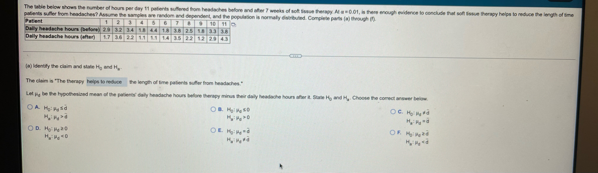
The table below shows the number of hours per day 11 patients suffered from headaches before and after 7 weeks of soft tissue therapy. At a=0.01, is there enough evidence to conclude that soft tissue therapy helps to reduce the length of time patients suffer from headaches? Assume the samples are random and dependent, and the population is normally distributed. Complete parts (a) through (). Patient Daily headache hours (before) 2.9 3.2 3.4 1.8 4.4 1.8 3.8 2.5 1.8 3.3 3.8 Daily headache hours (after) 1 2 3 4 56 789 10 11 0 1.7 3.6 2.2 1.1 1.1 1.4 3.5 2.2 12 2.9 4.3 (a) Identify the claim and state Ho and H The claim is "The therapy helps to reduce the length of time patients suffer from headaches." Let Ha be the hypothesized mean of the patients' daily headache hours before therapy minus their daily headache hours after it. State Ho and H Choose the correct answer below. OA. Ho: Ha sd O B. Ho: H s0 OC. Ho: Pad OD. Ho: Ha20 OE. Ho: Ma"d OF. Ho: Pa zd 0> Prt :"H

Compute the value of the test statistic and conclude.

J In-shop othesis test for the difference between two population proportions 02562 2600368.qx3zqy7 Jump to level 1 The manager of a coffee shop is trying to determine if drive-through customers buy fewer items than customers who come into the shop. The manager randomly samples both populations and calculates the proportion of customers in each that buy three or more items. The results of the data collected are shown below. What are the population parameters? Y Pick Drive-through Successes 27 Successes What is the level of significance? Ex: 0.12 Observations 76 Observations 41 119 0.345 p-hat_1 0.355 p-hat_2 What is the null hypothesis Ho? Pick Confidence Level 0.1429 What is the alternative hypothesis Ha? Pick p-value Should Ho be rejected or does Ho fail to be rejected? Pick What conclusion can be drawn from the data? Pick evidence exists to support the claim that drive-through customers buy fewer items than in-shop customers. 2 p W

The weight of a car can influence the mileage that the car can obtain. A random sample of 19 cars was taken and the weight (in pounds) and mileage (in mpg) were recorded and are in the table below. X, weight Y, mileage 2250 38.9 4500 17 4000 23.1 4500 19.5 3500 31.3 3500 31.3 3500 32.6 4000 23.4 4500 17.2 3500 28 5500 13.2 3500 28 2250 41.1 2500 40.9 2250 53.3 4000 23.6 3000 31.4 2750 46.9 3000 31.5 a) The symbol and value of the correlation coefficient are as follows:     Round final answer to 2 decimal places.     Select an answer r R² ρ ŷ y p̂ X̄ p μ σ s  =      Interpret this value: There is a strong Select an answer positive negative  Select an answer linear quadratic bell-shaped uniform  relation between weight and mileage for cars. b) The symbol and value of the coefficient of determination are as follows:     Round final answer to 2 decimal places.     Select an answer r r² ρ ŷ y p̂ X̄ p μ σ  =       Interpret this value: About…