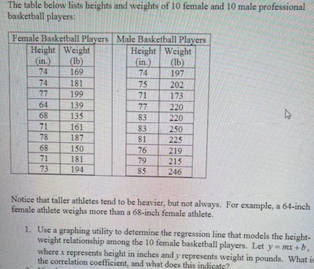
The table below lists heights and weights of 10 female and 10 male professional basketball players: Female Basketball Players Male Basketball Players Height Weight (in.) 74 Height (in.) Weight (lb) (Ib) 169 74 197 74 181 75 71 202 173 77 199 64 139 135 77 220 68 83 220 71 161 83 250 78 187 81 76 79 85 225 150 68 71 219 181 215 73 194 246 Notice that taller athletes tend to be heavier, but not always. For example, a 64-inch female athlete weighs more than a 68-inch female athlete. 1. Use a graphing utility to determine the regression line that models the height- weight relationship among the 10 female basketball players. Let y-mx +b, where x represents height in inches and y represents weight in pounds. Whati the correlation coefficient, and what docs this indigate?

I'm getting that the B is incorrect. Thank you for writing this out so I can go over and practice.

Please help me answer the following questions. Thank you

Preliminary data analysis indicate that it is reasonable to use a -test to carry out the specified hypothesis test. Perform the -test using the critical-value approach. a = 0.05 to test the claim that µ+35.8. The sample Use a significance level of data consists of 10 scores for which x=44.2 and s=7.3. Ho : µ±44.2 Η : μ 44.2 Test statistic: t= 3.64. Critical values: t=±2.262. Reject Ho : u=44.2. There is sufficient evidence to support the claim that the mean is different from 44.2. HO : μ-35.8 H : u#35.8 Test statistic: t=3.64. Critical values: t=±2.262. Reject Ho : u= 35.8. There is sufficient evidence to support the claim that the mean is different from 35.8. Ho : µ+35.8 Η : μ-35.8 Test statistic: t= 3.64. Critical values: t=±2.262. Reject H, : µ= 35.8. There is sufficient evidence to support the claim that the mean is different from 35.8. H0: μ=44.2 H, : µ+44.2 Test statistic: t= 3.64. Critical values: t=±2.262. Reject H : u= 1=44.2. There is sufficient evidence to support the claim…

Here's another one. Help me please...

if the value of A changes in responce to the value of B, then b is the?