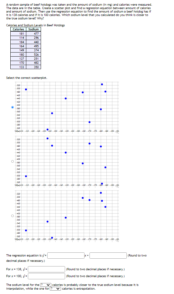
A random sample of beef hotdogs was taken and the amount of sodium (in mg) and calories were measured.The data are in the table. Create a scatter plot and find a regression equation between amount of caloriesand amount of sodium. Then use the regression equation to find the amount of sodium a beef hotdog has ifit is 138 calories and if it is 100 calories. Which sodium level that you calculated do you think is closer tothe true sodium level? Why?Calories and Sodium Levels in Beef HotdogsCaloriesSodium181477114296184440164495149374180526137251170482133350Select the correct scatterplot.500400440420400340300200124010 15 120 125 18015 140 145 150 155 100 45 170 175 Jao Jas I80 4p.500400440420400300340300200I4oio is 120 125 180 135 140 J45 J50 153 100 165 170o5004004404204003003403203002202001240lio is 120 125 180 1 140 145 150 155 100 165 170 175 Jao Jas J0 4s.The regression equation is y=decimal places if necessary.)(Round to twoFor x = 138, y=(Round to two decimal places if necessary.)For x = 100, y =(Round to two decimal places ff necessary.)The sodium level for the ?interpolation, while the one for ?v calories is probably closer to the true sodium level because it isv calories is extrapolation.

Answer: Scatter plot Option 3 is correct

Answered: The regression equation is y (Round to…

MATLAB: An Introduction with Applications

6th Edition

ISBN:9781119256830

Author:Amos Gilat

Publisher:Amos Gilat

Chapter1: Starting With Matlab

Section: Chapter Questions

Problem 1P

See similar textbooks

Similar questions

The table shows the amounts of crude oil (in thousands of barrels per day) produced by a certain country and the amounts of crude oil (in thousands of barrels per day) imported by the same country for seven years. The equation of the regression line is y=-1.196x+16,255.09. Complete parts (a) and (b) below. Produced, x Imported, y (a) Find the coefficient of determination and interpret the result (Round to three decimal places as needed.) How can the coefficient of determination be interpreted? The fraction of the variation in the amount of the variation is unexplained and is due to other factors or to sampling error. (b) Find the standard error of estimates, and interpret the result. thousands of barrels per day (Round to three decimal places as needed.) How can the standard error of estimate be interpreted? The standard error of estimate of the amount of 5,827 9,349 for 5,701 5,590 5410 5.216 5,105 5,035 9,107 9,654 10,059 10,105 10,198 10,003 BULLM that can be explained by the…
Need help If my outer regression equation is Weight= -191.891 + 5.06 (Height) How do I find the estimated weight LBS for an individual with height 76 inches?
Use the regression equation to predict the value of y= -2.8. Assume that the variable x and y have a significant
Given the regression equation Y = 43 - 10X, the predicted value of Y when X = -7 is O A. -113 O B. -70 O C. 113 O D. 70
The equation used to predict annual cauliflower yield (in pounds per acre) is y=24,596+4.423x1−4.772x2, where x1 is the number of acres planted an x2 is the number of acres harvested. Use the multiple regression equation to predict the y-values for the values of the independent variables.
Caselet #1 ADVERTISEMENT A marketing executive wishes to determine whether there is a relationship between the number of television commercials aired per week and the number of sales (in thousand pesos) of a product. The data for the sample follow. Number of Ads, x 2 8. 8. 10 12 Sales, y 2 4 7 6. 10
Please only answer “d” and “e” as I already have the other parts filled out. Thank you!
A regression analysis between cost to build a clinic (in dollars) and clinic size (in square foot) resulted in the following equation: y=75+6x. This implies that if the clinic size is 800 square feet, then the cost to build a clinic (in dollars) is?
The table shows the number of goals allowed and the total points earned (2 points for a win, and 1 point for an overtime or shootout loss) by 14 ice hockey teams over the course of a season. The equation of the regression line is ŷ= -0.556x+217.766. Use the data to answer the following questions. (a) Find the coefficient of determination, 12, and interpret the result. (b) Find the standard error of the estimate, Se, and interpret the result. 213 213 223 226 259 266 281 202 210 205 226 207 259 239 D Goals Allowed, x Points, y 109 109 102 91 88 80 52 105 107 98 95 85 68 66 (a)² = (Round to three decimal places as needed.) Interpret the coefficient of determination. Select the correct choice below and fill in the answer box to complete your choice. (Round to one decimal place as needed.) OA. About OB. About (b) Se = % of the variation in points earned can be explained by the relationship between number of goals allowed and points earned. The remaining variation is unexplained. % of the…
Given the regression equation Y = 43 - 10X, the change in Y when X changes by -3 is a. -13 O b. -30 Ос. 13 O. d. 30
What is the slope and intercept for the regression equation given this data?X = -5, 34, 56, 0, 61Y = 13, 63, 46, -23, 50
The regression equation of two variables are 3Y-2X 10 = 0 and 2Y-X-500. Find coefficient of correlation.

SEE MORE QUESTIONS

Recommended textbooks for you

MATLAB: An Introduction with Applications

Statistics

ISBN:

9781119256830

Author:

Amos Gilat

Publisher:

John Wiley & Sons Inc

Probability and Statistics for Engineering and th…

Statistics

ISBN:

9781305251809

Author:

Jay L. Devore

Publisher:

Cengage Learning

Statistics for The Behavioral Sciences (MindTap C…

Statistics

ISBN:

9781305504912

Author:

Frederick J Gravetter, Larry B. Wallnau

Publisher:

Cengage Learning

MATLAB: An Introduction with Applications

Statistics

ISBN:

9781119256830

Author:

Amos Gilat

Publisher:

John Wiley & Sons Inc

Probability and Statistics for Engineering and th…

Statistics

ISBN:

9781305251809

Author:

Jay L. Devore

Publisher:

Cengage Learning

Statistics for The Behavioral Sciences (MindTap C…

Statistics

ISBN:

9781305504912

Author:

Frederick J Gravetter, Larry B. Wallnau

Publisher:

Cengage Learning

Elementary Statistics: Picturing the World (7th E…

Statistics

ISBN:

9780134683416

Author:

Ron Larson, Betsy Farber

Publisher:

PEARSON

The Basic Practice of Statistics

Statistics

ISBN:

9781319042578

Author:

David S. Moore, William I. Notz, Michael A. Fligner

Publisher:

W. H. Freeman

Introduction to the Practice of Statistics

Statistics

ISBN:

9781319013387

Author:

David S. Moore, George P. McCabe, Bruce A. Craig

Publisher:

W. H. Freeman

SEE MORE TEXTBOOKS

The regression equation is y (Round to two decimal places if necessary.) For x 138, y (Round to two decimal places if necessary.) For x- 100, y- (Round to two decimal places if necessary.)