
MATLAB: An Introduction with Applications
6th Edition
ISBN: 9781119256830
Author: Amos Gilat
Publisher: John Wiley & Sons Inc
expand_more
expand_more
format_list_bulleted
Related questions
Question
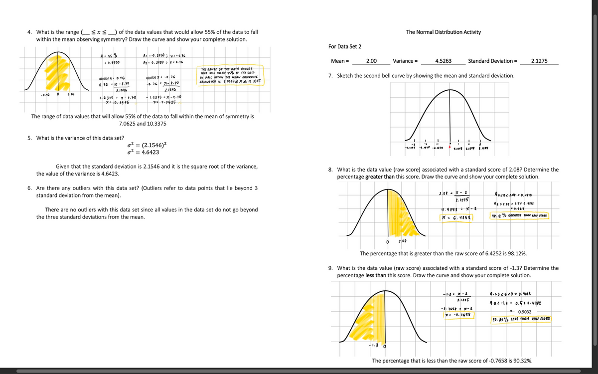

Transcribed Image Text:4. What is the range (sxs_) of the data values that would allow 55% of the data to fall
within the mean observing symmetry? Draw the curve and show your complete solution.
The Normal Distribution Activity
For Data Set 2
A. 4. 110 ;..16
A 0. 150 1G
..500
Mean =
2.000
Variance =
4.5263
Standard Deviation =
2.1275
THE RANGE OF THE DATA UALUES
7. Sketch the second bell curve by showing the mean and standard deviation.
UHEN -0,G
TO PALL n E MERN ORsrenNE
0.16 x-t.
. G A-t.t0
hart
1.6 315 : - t.10
** 10. 945
- 6SIS x-.10
11.0025
The range of data values that will allow 55% of the data to fall within the mean of symmetry is
7.0625 and 10.3375
5. What is the variance of this data set?
g? = (2.1546)?
g? = 4.6423
Given that the standard deviation is 2.1546 and it is the square root of the variance,
8. What is the data value (raw score) associated with a standard score of 2.08? Determine the
percentage greater than this score. Draw the curve and show your complete solution.
the value of the variance is 4.6423.
6. Are there any outliers with this data set? (Outliers refer to data points that lie beyond 3
standard deviation from the mean).
2.0r- X- 1
2.1215
Aocecior 0. vers
A1.0. .r .
There are no outliers with this data set since all values in the data set do not go beyond
the three standard deviations from the mean.
4.4151 X-
*. G. V252
r.12 o cereee T e eer
2.09
The percentage that is greater than the raw score of 6.4252 is 98.12%.
9. What is the data value (raw score) associated with a standard score of -1.3? Determine the
percentage less than this score. Draw the curve and show your complete solution.
-1.3.-1
2.1245
Aze -1.3 = 0.5+ D. v032
- 0.9032
*. -0. 165
90. 81, Lert HAN RAW SCoet
1.3 0
The percentage that is less than the raw score of -0.7658 is 90.32%.
Expert Solution
This question has been solved!
Explore an expertly crafted, step-by-step solution for a thorough understanding of key concepts.

This is a popular solution

Trending nowThis is a popular solution!

Step by stepSolved in 3 steps with 1 images

Follow-up Questions
Read through expert solutions to related follow-up questions below.
Follow-up Question
What is the
Solution
by Bartleby Expert
Follow-up Questions
Read through expert solutions to related follow-up questions below.
Follow-up Question
What is the
Solution
by Bartleby Expert
Knowledge Booster

Similar questions
- Page 2 of 5 B. Organizing and Working with Data. 1. Find the z-score for the weight of a 155-pound woman. The mean weight of woman age 20 or older is 170.6 pounds with a standard deviation of 5.4 pounds. Round your answer to two decimal places.arrow_forwardThe ratings of applicants for credit are normally distributed with a mean of 200 and a standard deviation of 50. Find the 60th. percentile, the rating score that separates the lower 60% from the top 40%. Round to the nearest integer. a. 208 b. 187 c. 211 d. 213arrow_forwardDetermine the number of standard deviations from the mean (z-score). In the United States, the distribution of a male's height has a mean of 69 inches with a standard deviation of 3 inches. How many standard deviations from the mean is John Doe, who is 67 inches tall? Question 15 options: 0.67 standard deviations below the mean 0.33 standard deviations below the mean 2 standard deviations below the mean 1 standard deviation below the meanarrow_forward
- Please do only sub-part "d" for Q6 and also do only sub-part "d" for Q9. Don't use excel formula to solve the question.arrow_forwardRefer to the data set in the accompanying table. Assume that the paired sample data is a simple random sample and the differences have a distribution that is approximately normal. Use a significance level of 0.05 to test for a difference between the weights of discarded paper (in pounds) and weights of discarded plastic (in pounds). E Click the icon to view the data. In this example, Hg is the mean value of the differences d for the population of all pairs of data, where each individual difference d is defined as the weight of discarded paper minus the weight of discarded plastic for a household. What are the null and alternative hypotheses for the hypothesis test? O A. Ho: Ha = 0 H,: Ha #0 O B. Ho: Ha #0 H1: Hd =0 O C. Ho: Ha #0 O D. Ho: Ha = 0 H1: Hd 0arrow_forwardAssume that a randomly selected subject is given a bone density test. Those test scores are normally distributed with a mean of 0 and a standard deviation of 1. Find the probability that a given score is between -2.05 and 3.87 and draw a sketch of the region. Sketch the region. Choose the correct graph below. OA. OB. OC. OD. -2.05 3.87 2.05 3.87 -2.05 3.87 -2.05 3.87 The probability is (Round to four decimal places as needed.)arrow_forward
- I need help answering parts 4 and 5arrow_forwardSuppose that the distance of fly balls hit to the outfield (in baseball) is normally distributed with a mean of 250 feet and a standard deviation of 48 feet. We randomly sample 49 fly balls. Part A. B. C. are listed in the included images.arrow_forwardAssume that a randomly selected subject is given a bone density test. Those test scores are normally distributed with a mean of 0 and a standard deviation of 1. Draw a graph and find the probability of a bone density test score greater than -3.71. Sketch the region. Choose the correct graph below. OA. 3.71 Q B. -3.71 The probability of a bone density test score greater than -3.71 is ☐. (Round to four decimal places as needed.) ๘ ๘ ปี OC. OD. Л 3.71 3.71arrow_forward
arrow_back_ios
arrow_forward_ios
Recommended textbooks for you
- MATLAB: An Introduction with ApplicationsStatisticsISBN:9781119256830Author:Amos GilatPublisher:John Wiley & Sons Inc
 Probability and Statistics for Engineering and th...StatisticsISBN:9781305251809Author:Jay L. DevorePublisher:Cengage Learning
 Statistics for The Behavioral Sciences (MindTap C...StatisticsISBN:9781305504912Author:Frederick J Gravetter, Larry B. WallnauPublisher:Cengage Learning
  Elementary Statistics: Picturing the World (7th E...StatisticsISBN:9780134683416Author:Ron Larson, Betsy FarberPublisher:PEARSON
 The Basic Practice of StatisticsStatisticsISBN:9781319042578Author:David S. Moore, William I. Notz, Michael A. FlignerPublisher:W. H. Freeman
 Introduction to the Practice of StatisticsStatisticsISBN:9781319013387Author:David S. Moore, George P. McCabe, Bruce A. CraigPublisher:W. H. Freeman
MATLAB: An Introduction with Applications
Statistics
ISBN:9781119256830
Author:Amos Gilat
Publisher:John Wiley & Sons Inc
Probability and Statistics for Engineering and th...
Statistics
ISBN:9781305251809
Author:Jay L. Devore
Publisher:Cengage Learning
Statistics for The Behavioral Sciences (MindTap C...
Statistics
ISBN:9781305504912
Author:Frederick J Gravetter, Larry B. Wallnau
Publisher:Cengage Learning
Elementary Statistics: Picturing the World (7th E...
Statistics
ISBN:9780134683416
Author:Ron Larson, Betsy Farber
Publisher:PEARSON
The Basic Practice of Statistics
Statistics
ISBN:9781319042578
Author:David S. Moore, William I. Notz, Michael A. Fligner
Publisher:W. H. Freeman
Introduction to the Practice of Statistics
Statistics
ISBN:9781319013387
Author:David S. Moore, George P. McCabe, Bruce A. Craig
Publisher:W. H. Freeman