
MATLAB: An Introduction with Applications
6th Edition
ISBN: 9781119256830
Author: Amos Gilat
Publisher: John Wiley & Sons Inc
expand_more
expand_more
format_list_bulleted
Related questions
Question
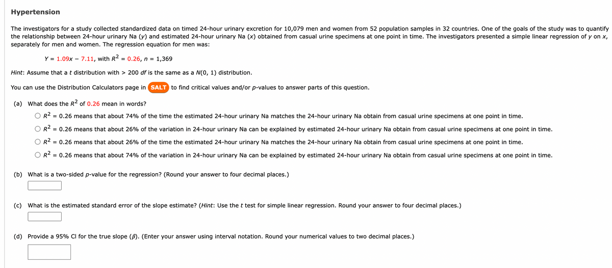

Transcribed Image Text:Hypertension
The investigators for a study collected standardized data on timed 24-hour urinary excretion for 10,079 men and women from 52 population samples in 32 countries. One of the goals of the study was to quantify
the relationship between 24-hour urinary Na (y) and estimated 24-hour urinary Na (x) obtained from casual urine specimens at one point in time. The investigators presented a simple linear regression of y on x,
separately for men and women. The regression equation for men was:
Y = 1.09x - 7.11, with R² = 0.26, n = 1,369
Hint: Assume that a t distribution with > 200 df is the same as a N(0, 1) distribution.
You can use the Distribution Calculators page in SALT to find critical values and/or p-values to answer parts of this question.
(a) What does the R² of 0.26 mean in words?
R²:
= 0.26 means that about 74% of the time the estimated 24-hour urinary Na matches the 24-hour urinary Na obtain from casual urine specimens at one point in time.
R² = 0.26 means that about 26% of the variation in 24-hour urinary Na can be explained by estimated 24-hour urinary Na obtain from casual urine specimens at one point in time.
R² = 0.26 means that about 26% of the time the estimated 24-hour urinary Na matches the 24-hour urinary Na obtain from casual urine specimens at one point in time.
OR²
= 0.26 means that about 74% of the variation in 24-hour urinary Na can be explained by estimated 24-hour urinary Na obtain from casual urine specimens at one point in time.
(b) What is a two-sided p-value for the regression? (Round your answer to four decimal places.)
(c) What is the estimated standard error of the slope estimate? (Hint: Use the t test for simple linear regression. Round your answer to four decimal places.)
(d) Provide a 95% CI for the true slope (B). (Enter your answer using interval notation. Round your numerical values to two decimal places.)

Transcribed Image Text:The actual regression equation used to derive the estimated 24-hour urinary Na for men in North America also included several additional variables and was as follows.
Multiple linear regression of 24-hour
urinary Na on casual urinary measurements
and other risk factors
Variable
Intercept
Casual Na (mmol/L)
Casual creatinine (mmol/L)
Casual potassium (mmol/L)
Body mass index (kg/m²)
Age (years)
Age² (years²)
Beta
25.42 16.65
0.42
-2.71
-0.12
=
se
0.28
0.00
0.02
0.26
4.16 0.35
0.05
0.76
0.01
(e) What does the regression coefficient for casual potassium (-0.12) mean in words?
The regression coefficient of -0.12 means that for every 1 mmol/L increase in casual urinary potassium, there is an expected decrease of 0.12 mmol/L in 24-hour urinary Na regardless of whether
other factors are changing along with casual urinary potassium.
The regression coefficient of -0.12 means that for every 1 mmol/L increase in casual urinary potassium, there is an expected increase of 0.12 mmol/L in 24-hour urinary Na, holding all other factors
in the multiple regression equation constant.
The regression coefficient of -0.12 means that for every 1 mmol/L increase in casual urinary potassium, there is an expected increase of 0.12 mmol/L in 24-hour urinary Na regardless of whether
other factors are changing along with casual urinary potassium.
The regression coefficient of -0.12 means that for every 1 kg/m² increase in casual urinary potassium, there is an expected decrease of 0.12 kg/m² in 24-hour urinary Na, holding all other factors in
the multiple regression equation constant.
The regression coefficient of -0.12 means that for every 1 mmol/L increase in casual urinary potassium, there is an expected decrease of 0.12 mmol/L in 24-hour urinary Na, holding all other factors
in the multiple regression equation constant.
(f) Provide a two-sided p-value associated with the regression coefficient for casual potassium (-0.12). (Round your answer to four decimal places.)
p-value
Provide a 95% Cl associated with the regression coefficient for casual potassium (-0.12). (Enter your answer using interval notation. Round your numerical values to two decimal places.)
Expert Solution
This question has been solved!
Explore an expertly crafted, step-by-step solution for a thorough understanding of key concepts.

This is a popular solution

Trending nowThis is a popular solution!

Step by stepSolved in 5 steps with 18 images

Knowledge Booster

Similar questions
- Low-Density Lipoprotein (or LDL) is considered the "bad" cholesterol because it forms plaques in arteries, raising the risk for heart attack and stroke. Suppose you are interested in predicting LDL (in mg/dL) using one's age (in years). Assume that LDL levels and age are normally distributed and that the correlation between the two variables is 0.534. Based solely on the regression effect, a person whose age is at the 60th percentile is predicted to have an LDL level ____. [Source: Ldl cholesterol: Definition, risks, and how to lower it. (2020, March 09). Retrieved from https://www.webmd.com/heart-disease/ldl-cholesterol-the-bad-cholesterol] Question 4 options: A) above the 60th percentile B) exactly at the 60th percentile C) exactly at the 40th percentile D) I need more information to answer this E) below the 60th percentilearrow_forwardThe following table shows the starting salary and profile of a sample of 10 2 p employees in a certain call center agency. Run a multiple regression analysis with starting salary as the dependent variable (pesos) and GPA, years of experience and civil service ratings as the independent variables. Use .05 level of significance.What is the computed R square of the resulting multiple linear regression and its interpretation? * Civil Years of Starting salary GPA service experience ratings 79.5 15000 80.1 15000 81.2 78.0 15500 81.3 79.0 16000 82.4 80.0 16200 83.4 85.0 17500 87.9 89.9 89.1 18000 90.3 16,300 84.2 17000 87.0 17900 88.1 84.1 89.0 89.2 R squared = 0.8053; This means that 80.53% of the total variation in the starting salary can be explained by its linear relationship with GPA, years of experience and civil service ratings. R squared = 0.9651; This means that 96.51% of the total variation in the starting salary can be explained by its linear relationship with GPA, years of…arrow_forwardIn a sample of cars reviewed by Motor Trend magazine, the mean horsepower (hp) was 150 hp with a standard deviation of 36 hp. The mean weight (lbs) was 2500 lbs with a standard deviation of 720 lbs. Assume the relationship between weight and horsepower is linear and has a correlation of r = +0.55. What is the slope of the linear regression model predicting weight (y-variable) from horsepower (x-variable)? 9 13 15 11arrow_forward
- A small independent organic food store offers a variety of specialty coffees. To determine whether price has an impact on sales, the managers kept track of how many kilograms of each variety of coffee were sold last month. The data and summary statistics (including the averages, standard deviations and the correlation coefficient) are shown in the table. If the "price per kilogram" is the predictor variable and "kilograms sold" is the response variable, then use a regression line to predict the the amount of kilograms sold for a "price per kilogram" equal to $15. Round your numbers to 3 decimal places.arrow_forwardThe value of PRESS for five different regression models are A = 42.3, B = 47.4, C = 51.5, D =40.6, and E = 54.6. Based only on this statistic, which model is preferred?arrow_forwardThe Wall Street Journal asked Concur Technologies, Inc., an expense management company, to examine data from million expense reports to provide insights regarding business travel expenses. Their analysis of the data showed that New York was the most expensive city. The following table shows the average daily hotel room rate () and the average amount spent on entertainment () for a random sample of of the most-visited U.S. cities. These data lead to the estimated regression equation . For these data . Click on the datafile logo to reference the data. Use Table 1 of Appendix B. full question attached in ss thanks for help aprpeicated aigjrowoirjarrow_forward
arrow_back_ios
arrow_forward_ios
Recommended textbooks for you
- MATLAB: An Introduction with ApplicationsStatisticsISBN:9781119256830Author:Amos GilatPublisher:John Wiley & Sons Inc
 Probability and Statistics for Engineering and th...StatisticsISBN:9781305251809Author:Jay L. DevorePublisher:Cengage Learning
 Statistics for The Behavioral Sciences (MindTap C...StatisticsISBN:9781305504912Author:Frederick J Gravetter, Larry B. WallnauPublisher:Cengage Learning
  Elementary Statistics: Picturing the World (7th E...StatisticsISBN:9780134683416Author:Ron Larson, Betsy FarberPublisher:PEARSON
 The Basic Practice of StatisticsStatisticsISBN:9781319042578Author:David S. Moore, William I. Notz, Michael A. FlignerPublisher:W. H. Freeman
 Introduction to the Practice of StatisticsStatisticsISBN:9781319013387Author:David S. Moore, George P. McCabe, Bruce A. CraigPublisher:W. H. Freeman
MATLAB: An Introduction with Applications
Statistics
ISBN:9781119256830
Author:Amos Gilat
Publisher:John Wiley & Sons Inc
Probability and Statistics for Engineering and th...
Statistics
ISBN:9781305251809
Author:Jay L. Devore
Publisher:Cengage Learning
Statistics for The Behavioral Sciences (MindTap C...
Statistics
ISBN:9781305504912
Author:Frederick J Gravetter, Larry B. Wallnau
Publisher:Cengage Learning
Elementary Statistics: Picturing the World (7th E...
Statistics
ISBN:9780134683416
Author:Ron Larson, Betsy Farber
Publisher:PEARSON
The Basic Practice of Statistics
Statistics
ISBN:9781319042578
Author:David S. Moore, William I. Notz, Michael A. Fligner
Publisher:W. H. Freeman
Introduction to the Practice of Statistics
Statistics
ISBN:9781319013387
Author:David S. Moore, George P. McCabe, Bruce A. Craig
Publisher:W. H. Freeman