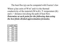
The heat flux (q) can be computed with Fourier's law Where q has units of W/m2 and k is the thermal conductivity of the material (W/m.K). T: temperature (K) and x = distance (m) along the path of heat flow. Determine at each point for the following data using the best finite divided approximation formulas. x (cm)T (K) 10 800 15 760 630 25 480 35 370 40 300 55 200 70

Using AutoCAD or any other software, draw front and right-side views from below using offset sections (as shown from the top view below). 1:1 scale use 3rd angle view (American projection) and dimensions included. 85 24 56 10 40 22 22 4.5 R2 R6 R3 24 20 46 95 TOP VIEW 36 6XM6 6.5 ン ず 8L

Question 8 and 9

Q1. Honey is a very widely used ingredient in cooking all around the world. Many commercial honey manufacturers heat treat honey to remove harmful bacteria that may be present. The density and viscosity of the honey varies with temperature, as shown in table 1. Temperature K 293 298 303 308 313 318 323 Density kg/m³ 1403 1398 1393 1388 1383 1378 1373 Viscosity Pas 55.66 46.45 37.99 30.28 23.32 17.11 11.65 Table 1: Fluid properties of honey. A particular processing facility heats and sterilises 500 kg of unprocessed honey every 30 minutes. The unpro- cessed honey is stored in large vats, then pumped though pipes into heating units before being pumped through another pipe to be bottled. The pipe carrying the honey from a storage container, which is 11 m tall, to a heating unit is 5 m long and has a diameter of 10 cm. Prior to being heated the honey is kept at 25°C. (a) What is the pressure difference between the top and bottom of a storage vat when it is full? (b) What is the volume flow…

Q1

You are designing a spherical tank to hold water for a small village. The volume of liquid it can hold can be computed as V = nh?(3R=h) %3D where V = volume [m³], h = depth of water in tank [m], and R = the tank radius [m]. Use Newton Raphson method with 1 iterations to find the relative percentage error in height calculation (e = 100|(hi+1 – hi)/h;) for storing 20 m³ of water with 10 m diameter-tank. Take T = 3.1416 and initial guess for h=R. %3D %3D Choices 61.5737 60.3422 30.7869 92.3606 Submit I Attempts 1 2 |

In your biomechanical testing lab, you perform a series of compression tests to determine the relationship between apparent bone density (p, units of g/cm³) and ultimate stress (ơult, units of MPa). Using the set of experimental measurements below, write an m-file to fit a power relationship of the form O uli = Ap to the data. Use the log transform method to linearize the system and data, followed by linear regression. Plot the data points and the power relationship on a single plot. Be sure to label your axes and provide a legend. Provide a printout of your m-file and a printout of the command window showing your results. Write down the best fit equation and box it. 8.76 5.25 4.26 5.51 3.88 18.45 2.09 13.72 5.42 2.17 Oult (MPa) p (g/cm³) 0.598 | 0.459 0.319 | 0.235 0.141 0.754 0.177 0.553 0.394 0.246