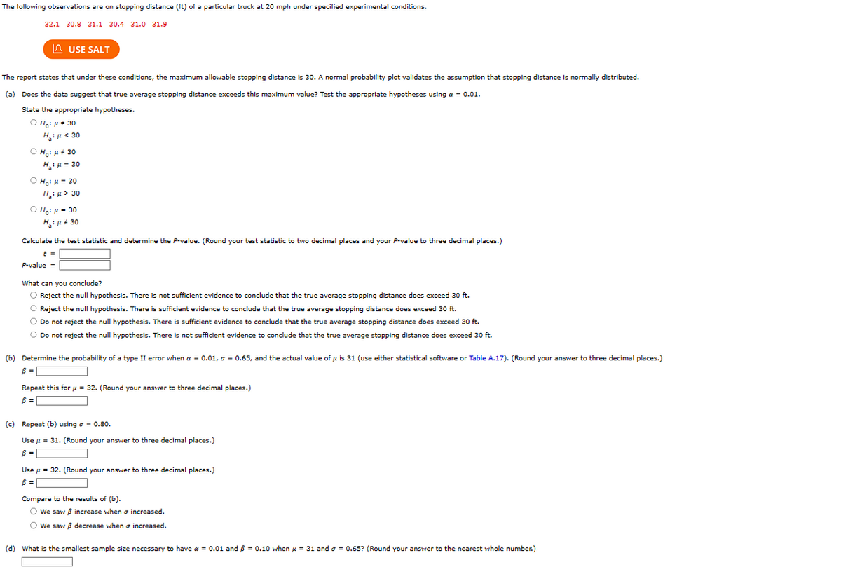
The following observations are on stopping distance (ft) of a particular truck at 20 mph under specified experimental conditions. 32.1 30.8 31.1 30.4 31.0 31.9 USE SALT The report states that under these conditions, the maximum allowable stopping distance is 30. A normal probability plot validates the assumption that stopping distance is normally distributed. (a) Does the data suggest that true average stopping distance exceeds this maximum value? Test the appropriate hypotheses using a = 0.01. State the appropriate hypotheses. ⒸHO: 30 H₂:μ < 30 ⒸHO: #30 H₁:μ= 30 ⒸH₂: μ = 30 H₂:μ> 30 ⒸHO: H = 30 H₂:μ* 30 Calculate the test statistic and determine the P-value. (Round your test statistic to two decimal places and your P-value to three decimal places.) P-value What can you conclude? O Reject the null hypothesis. There is not sufficient evidence to conclude that the true average stopping distance does exceed 30 ft. O Reject the null hypothesis. There is sufficient evidence to conclude that the true average stopping distance does exceed 30 ft. O Do not reject the null hypothesis. There is sufficient evidence to conclude that the true average stopping distance does exceed 30 ft. =

Expected returns and standard deviations have been calculated for five projects. Rank them in terms of total risk, from highest risk to lowest risk. std deviation Project A B C D E O DACBE O AEDCB O EDBCA O ACEBD O none of these E(R) 5.9% 12.3% 8.4% 14.9% 16.2% 1.8% 2.5% 2.3% 2.9% 3.3%

Consider the following data from a repeated-measures design. You want to use a repeated-measures t test to test the null hypothesis Ho: HD = 0 (the null hypothesis states that the mean difference for the general population is zero). The data consist of five observations, each with two measurements, A and B, taken before and after a treatment. Assume the population of the differences in these measurements are normally distributed. A B Observation 1 1 3 4 3 7 4 4 4 5 8 9 You conduct a two-tailed test at a = .05. To find the critical value (in the table) you first need to get the degrees of freedom, which is The critical values (the values for t-scores that separate the tails from the main body of the distribution, forming the critical region) are = Based on this our finding v significant and we the null hypothesis.

Chebyshev's theorem Student. d major university are complaining of a serious housing crunch. Many of the university's students, they complain, have to commute too far to school because there is not enough housing near campus. The university officials respond with the following Information: the mean distance commuted to school by students is 14.7 miles, and the standard deviation of the distance commuted is 3.1 miles. Assuming that the university officials' Information is correct, complete the following statements about the distribution of commute distances for students at this university. (a) According to Chebyshev's theorem, at least 36% of the commute distances lie between miles and miles. (Round your answer to 1 decimal 图 place.) ?. (b) According to Chebyshev's theorem, at least 7 of the commute distances lie between 8.5 miles and 20.9 miles. Explanation Check 2021 McGraw-H Al Rights eserved Te of ne Priry Acces 7. e S d CO alt ctri alt USE YOUR SMARTPMOW Chromebook x360…

TABLE 12-11 A computer software developer would like to use the number of downloads (in thousands) for the trial version of his new shareware to predict the amount of revenue (in thousands of dollars) he can make on the full version of the new shareware. Following is the output from a simple linear regression along with the residual plot and normal probability plot obtained from a data set of 30 different sharewares that he has developed: Regression Statistics Multiple R R Square Adjusted R Square Standard Error Observations 0.8691 0.7554 0.7467 44.4765 30.0000 ANOVA Significance F 0.0000 df SS 171062.9193 171062.9193 MS Regression Residual 86.4759 28 55388.4309 1978. 1582 Total 29 226451.3503 Standard Error 26.9183 0.4011 P-value Intercept Download Coefficients 95.0614 3.7297 t Stat 3.5315 9.2992 0.0015 0.0000 Lower 95% -150, 2009 Upper 95% 39.9218 2.9082 4.5513 Download Residual Plot 120 100 80 60 40 20 -20 -40 -60 -80 100 20.00 60.00 80.00 100.00 120.00 0.00 40.00 Download Normal…

Determine if the finite correction factor should be used. If​ so, use it in your calculations when you find the probability. In a sample of  900 gas​ stations, the mean price for regular gasoline at the pump was $2.889 per gallon and the standard deviation was ​$0.009 per gallon. A random sample of size 60 is drawn from this population. What is the probability that the mean price per gallon is less than ​$2.886��?

Determine if the finite correction factor should be used. If​ so, use it in your calculations when you find the probability. In a sample of 800 gas​ stations, the mean price for regular gasoline at the pump was $2.869 per gallon and the standard deviation was ​$0.008 per gallon. A random sample of size 45 is drawn from this population. What is the probability that the mean price per gallon is less than ​$2.867​?