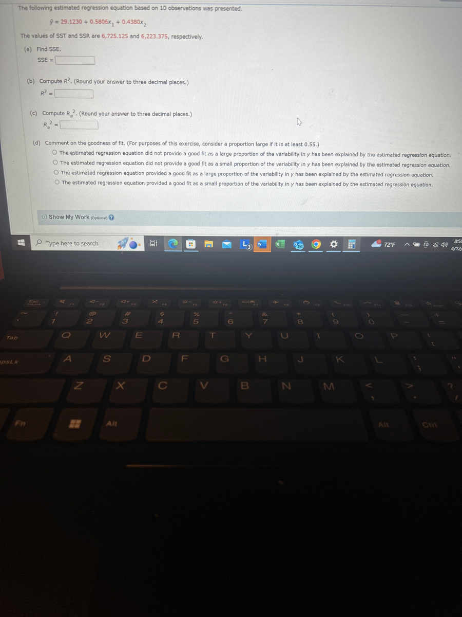
The following estimated regression equation based on 10 observations was presented. ŷ= 29.1230+ 0.5806x + 0.4380x2 The values of SST and SSR are 6,725.125 and 6,223.375, respectively. (a) Find SSE. SSE= (b) Compute R2. (Round your answer to three decimal places.) R² = (c) Compute R. (Round your answer to three decimal places.) R2= (d) Comment on the goodness of fit. (For purposes of this exercise, consider a proportion large if it is at least 0.55.) O The estimated regression equation did not provide a good fit as a large proportion of the variability in y has been explained by the estimated regression equation. O The estimated regression equation did not provide a good fit as a small proportion of the variability in y has been explained by the estimated regression equation. O The estimated regression equation provided a good fit as a large proportion of the variability in y has been explained by the estimated regression equation. O The estimated regression equation provided a good fit as a small proportion of the variability in y has been explained by the estimated regression equation. Tab Esc Show My Work (Optional) Type here to search 1 40+ @ #f $ % & 3 4 5 6 7 8 O W E R T A S D F G H J K psLk N x C B N M Fn Alt 72°F 8:50 4/12/ Alt Ctri

A regression was run to determine if there is a relationship between hours of TV watched per day, x, and number of sit-ups, y, a person can do in a minute. The results of the regression were: y=ax+b a=-1.255 b=21.239 Use this to predict the number of sit-ups a person who watches 11.5 hours of TV can do in a minute. Round to the nearest whole number.

A regression was run to determine if there is a relationship between hours of TV watched per day (x) and the number of sit-ups a person can do (y). The results were: Y a+bx b = -0.79 = 23.04 a r² = 0.4493 r = -0.6703 a. If a person watches 10 hours of television a day, predict how many sit-ups he can do. b. If a person can do 7 sit ups, predict how many hours of television a day they watch. hours

Suppose that you want to compare the means of several treatments in a randomized block ANOVA. If given the choice between using the randomized block ANOVA test and the Friedman test, which one would you choose if outliers occur in the sample data? Explain your answer.

A regression was run to determine if there is a relationship between hours of TV watched per day (x) and number of situps a person can do (y). The results of the regression were: y=a+bx b=-0.993 a=29.135 r2=0.463761 r=-0.681 Use this to predict the number of situps a person who watches 6 hours of TV can do. Round to one decimal place.

A regression analysis was performed to determine if there is a relationship between hours of TV watched per day () and number of sit ups a person can do (y). The results of the regression were: y=ax+b a=-1.153 b=22.899 r2=0.649636 r=-0.806 Use this to predict the number of sit ups a person who watches 8 hours of TV can do, and please round your answer to a whole number.