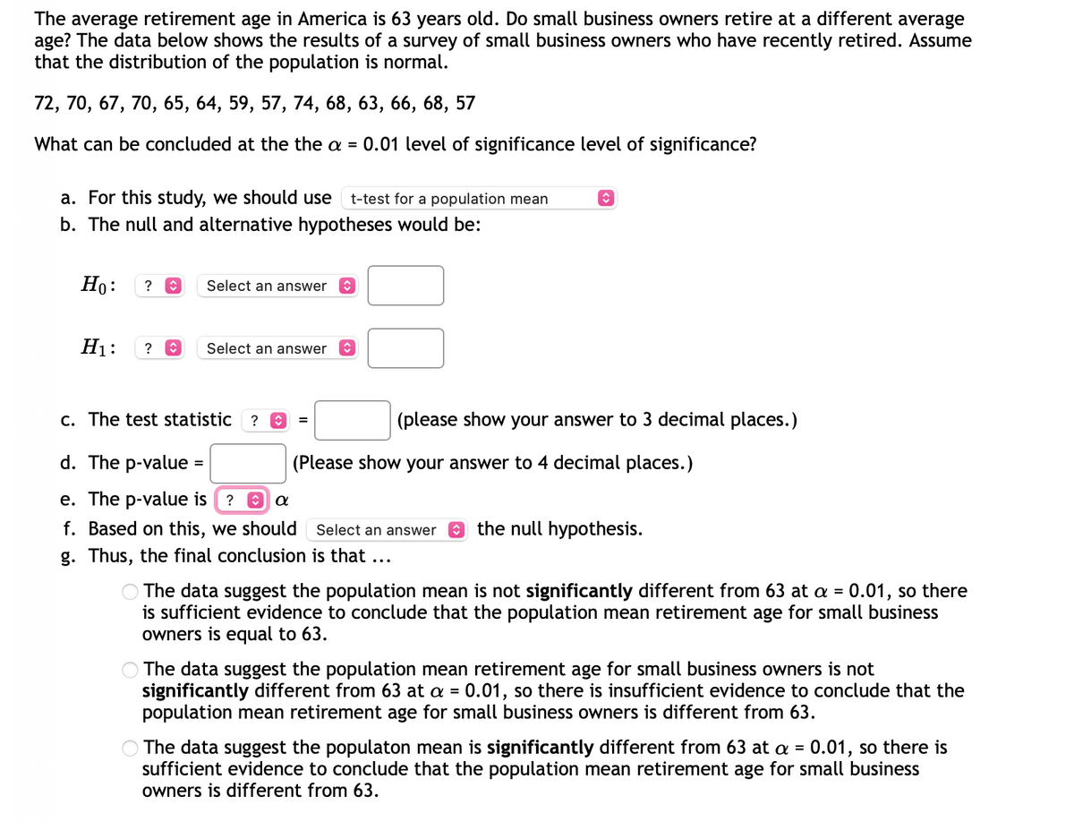
The average retirement age in America is 63 years old. Do small business owners retire at a different average age? The data below shows the results of a survey of small business owners who have recently retired. Assume that the distribution of the population is normal. 72, 70, 67, 70, 65, 64, 59, 57, 74, 68, 63, 66, 68, 57 What can be concluded at the the a = 0.01 level of significance level of significance? a. For this study, we should use t-test for a population mean b. The null and alternative hypotheses would be: Ho: ? Select an answer î H₁: ? î Select an answer c. The test statistic ? = (please show your answer to 3 decimal places.) d. The p-value = (Please show your answer to 4 decimal places.) e. The p-value is ? Εα f. Based on this, we should Select an answer the null hypothesis. g. Thus, the final conclusion is that ... O The data suggest the population mean is not significantly different from 63 at a = 0.01, so there is sufficient evidence to conclude that the population mean retirement age for small business owners is equal to 63. The data suggest the population mean retirement age for small business owners is not significantly different from 63 at a = 0.01, so there is insufficient evidence to conclude that the population mean retirement age for small business owners is different from 63. O The data suggest the populaton mean is significantly different from 63 at a = 0.01, so there is sufficient evidence to conclude that the population mean retirement age for small business owners is different from 63.

The average house has 14 paintings on its walls. Is the mean larger for houses owned by teachers? The data show the results of a survey of 14 teachers who were asked how many paintings they have in their houses. Assume that the distribution of the population is normal. 15, 13, 16, 16, 17, 14, 14, 15, 13, 13, 15, 16, 15, 16 What can be concluded at the a = 0.01 level of significance? a. For this study, we should use Select an answer b. The null and alternative hypotheses would be: Но: ? Select an answer v H: ?v Select an answer v c. The test statistic ? v = (please show your answer to 3 decimal places.) d. The p-value = (Please show your answer to 4 decimal places.) e. The p-value is ? va f. Based on this, we should Select an answer v the null hypothesis. g. Thus, the final conclusion is that ... O The data suggest that the population mean number of paintings that are in teachers' houses is not significantly more than 14 at a = 0.01, so there is insufficient evidence to conclude that…

2. The test scores of 16 students are listed below: 44, 46, 51, 57, 60, 63, 65, 70, 75, 76, 85, 87, 90, 94, 95, 97. (c) Find the third quartile of the above data. 87 88.5 57 58.5

Do rats take less time on average than hamsters to travel through a maze? The table below shows the times in seconds that the rats and hamsters took. Rats: 36, 35, 22, 42, 25, 14, 31, 14 Hamsters: 41, 37, 12, 46, 39, 46, 38, 45, 27, 29 Assume that both populations follow a normal distribution. What can be concluded at the a = 0.05 level of significance level of significance? For this study, we should use Select an answer a. The null and alternative hypotheses would be: Ho: Select an answer v Select an answer v Select an answer v (please enter a decimal) H: Select an answer v Select an answer v Select an answer v (Please enter a decimal) b. The test statistic (please show your answer to 3 decimal places.) c. The p-value = (Please show your answer to 4 decimal places.) d. The p-value is ? ♥ a e. Based on this, we should Select an answer f. Thus, the final conclusion is that ... the null hypothesis. O The results are statistically insignificant at a = 0.05, so there is statistically…

A random sample of 25 Berkeley College students was asked, “How many hours per week typically do you work outside the home?” Their responses were as follows: {0, 0, 15, 20, 30, 40, 30, 20, 35, 35, 28, 15, 20, 25, 25, 30, 5, 10, 30, 24, 28, 30, 35, 15, 15} a. Find the mean, the median and the mode of hours worked outside the home for the sample data. Show all your work to justify your answer. b. Use the above data to complete the following table summarizing the number of hours worked outside the home. Express the relative frequency as a percent. Class  Tally   Frequency    Relative Frequency  0-10 11-20 21-30 31-40 Total c. Find the five-number summary of the hours worked outside of the home by the 25 Berkeley College students.

2. Jim Miller works in the personnel department for a car company. He is told by his supervisor to investigate the difference in the average number of sick days between blue collar workers and whitecollar workers. So he obtained a random sample of 9 blue collar workers and a random sample of 9 white collar workers. He records the results below.At 10% level of significance, is there sufficient evidence to indicate a difference in mean sick days between blue collar workers and white collar workers.

The mean number of sick days an employee takes per year is believed to be about 10.5. Members of a personnel department do not believe this figure. They randomly survey ten employees. The number of sick days they took for the past year are as follows: 12; 4; 15; 3; 11; 8; 6; 8; 2; 9. Let x = the number of sick days they took for the past year. Should the personnel team believe that the mean number is ten?

Do rats take the same amount of time on average than hamsters to travel through a maze? The table below shows the times in seconds that the rats and hamsters took. Rats: 31, 26, 35, 34, 31, 39, 39, 6 Hamsters: 36, 35, 16, 29, 20, 25, 28, 37 Assume that both populations follow a normal distribution. What can be concluded at the a = 0.05 level of significance level of significance? For this studv, we should use Select an answer a. The null and alternative hypotheses would be: Ho: Select an answer v Select an answer v Select an answer V (please enter a decimal) H1: Select an answer v Select an answer v v (Please enter a decimal) Select an answer b. The test statistic ?v= (please show your answer to 3 decimal places.) c. The p-value = (Please show your answer to 4 decimal places.) d. The p-value is ? va e. Based on this, we should Select an answer v the null hypothesis. f. Thus, the final conclusion is that ... O The results are statistically insignificant at a = 0.05, so there is…

How many sources of between-group variation are measured in a two-way between-subjects ANOVA? Group of answer choices a. 4 b. 2 c. 3 d. 5

1. A furniture store reduces the prices of sofas in an autumn sale. The number of sofas sold during the 19 days of the sale were: 41, 44, 48, 55, 40, 44, 45, 42, 55, 55, 36, 36, 51, 47, 41, 38, 43, 48, 53 Work out the median and the lower and upper quartiles for the number of sofas sold in (3) the sale.