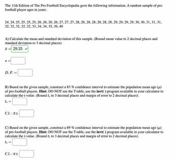
The 11th Edition of The Pro Football Encyclopedia gave the following information. A random sample of pro football player ages in years: 24, 24, 25, 25, 25, 25, 26, 26, 26, 26, 27, 27, 27, 28, 28, 28, 28, 28, 28, 28, 29, 29, 29, 29, 30, 30, 31, 31, 31, 32, 32, 32, 32, 32, 33, 34, 34, 35, 36, 40 A) Calculate the mean and standard deviation of this sample. (Round mean value to 2 decimal places and standard deviation to 3 decimal places) x = 29.25 ✓ S= D.F.= B) Based on the given sample, construct a 83 % confidence interval to estimate the population mean age (μ) of pro football players. Hint: DO NOT use the T-table, use the invt() program available in your calculator to calculate the t-value. (Round te to 3 decimal places and margin of error to 2 decimal places). tc C.I. : x C) Based on the given sample, construct a 89 % confidence interval to estimate the population mean age (μ) of pro football players. Hint: DO NOT use the T-table, use the invt() program available in your calculator to calculate the t-value. (Round te to 3 decimal places and margin of error to 2 decimal places). tc - C.I. : x

Definition Definition Measure of central tendency that is the average of a given data set. The mean value is evaluated as the quotient of the sum of all observations by the sample size. The mean, in contrast to a median, is affected by extreme values. Very large or very small values can distract the mean from the center of the data. Arithmetic mean: The most common type of mean is the arithmetic mean. It is evaluated using the formula: μ = 1 N ∑ i = 1 N x i Other types of means are the geometric mean, logarithmic mean, and harmonic mean. Geometric mean: The nth root of the product of n observations from a data set is defined as the geometric mean of the set: G = x 1 x 2 ... x n n Logarithmic mean: The difference of the natural logarithms of the two numbers, divided by the difference between the numbers is the logarithmic mean of the two numbers. The logarithmic mean is used particularly in heat transfer and mass transfer. ln x 2 − ln x 1 x 2 − x 1 Harmonic mean: The inverse of the arithmetic mean of the inverses of all the numbers in a data set is the harmonic mean of the data. 1 1 x 1 + 1 x 2 + ...