
MATLAB: An Introduction with Applications
6th Edition
ISBN: 9781119256830
Author: Amos Gilat
Publisher: John Wiley & Sons Inc
expand_more
expand_more
format_list_bulleted
Related questions
Question
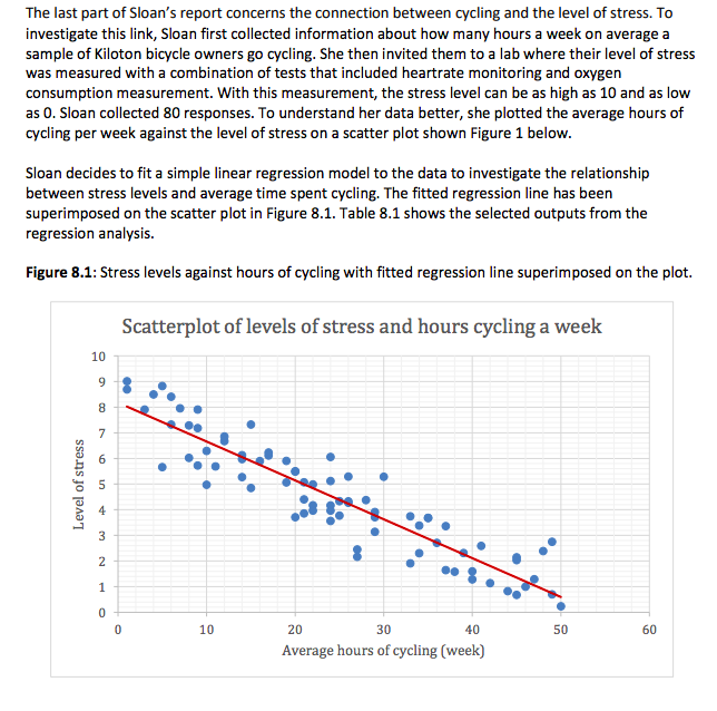

Transcribed Image Text:The last part of Sloan's report concerns the connection between cycling and the level of stress. To
investigate this link, Sloan first collected information about how many hours a week on average a
sample of Kiloton bicycle owners go cycling. She then invited them to a lab where their level of stress
was measured with a combination of tests that included heartrate monitoring and oxygen
consumption measurement. With this measurement, the stress level can be as high as 10 and as low
as 0. Sloan collected 80 responses. To understand her data better, she plotted the average hours of
cycling per week against the level of stress on a scatter plot shown Figure 1 below.
Sloan decides to fit a simple linear regression model to the data to investigate the relationship
between stress levels and average time spent cycling. The fitted regression line has been
superimposed on the scatter plot in Figure 8.1. Table 8.1 shows the selected outputs from the
regression analysis.
Figure 8.1: Stress levels against hours of cycling with fitted regression line superimposed on the plot.
Scatterplot of levels of stress and hours cycling a week
10
8.
7
6
4
3
1
10
20
30
40
50
60
Average hours of cycling (week)
Level of stress
9,

Transcribed Image Text:Table 8.1: Selected Excel output from a simple linear regression of levels of stress and average hours
of cycling a week; n=80
ANOVA
Significance
df
MS
F
Regression
1.
330.0887 330.0887 439.5926
8.61E-34
Residual
78
58.56994 0.750897
Total
79 388.6586
Standard
Coefficients
Error
t Stat
P-value
Intercept
Hours of cycling
8.174779154 0.201398 40.59015
<0.0001
(week)
-0.151563181 0.007229 -20.9665
<0.0001
By looking at the output in Table 8.1, write down the equation of the fitted regression model, and
explain the meaning of the regression coefficients in context. Comment on the statistical significance
of the regression coefficients.
Expert Solution
arrow_forward
Step 1
In this case, the independent variable is hours of cycling (x) and the dependent variable is levels of stress (y).

Step by stepSolved in 2 steps

Knowledge Booster

Similar questions
- Please see attached image for questionarrow_forwardConsider the following computer output of a multiple regression analysis relating annual salary to years of education and years of work experience. Regression Statistics Multiple R 0.73360.7336 R Square 0.53810.5381 Adjusted R Square 0.51800.5180 Standard Error 2140.27632140.2763 Observations 49 ANOVA dfdf SSSS MSMS F� Significance F� Regression 22 245,430,999.7671245,430,999.7671 122,715,499.8836122,715,499.8836 26.789226.7892 1.9E-081.9E-08 Residual 4646 210,716,007.0084210,716,007.0084 4,580,782.76114,580,782.7611 Total 4848 456,147,006.7755456,147,006.7755 Coefficients Standard Error t� Stat P-value Lower 95%95% Upper 95%95% Intercept 14276.146814276.1468 2,531.84252,531.8425 5.63865.6386 0.0000010040.000001004 9179.81229179.8122 19,372.481419,372.4814 Education (Years) 2349.95952349.9595 338.5500338.5500 6.94126.9412 0.0000000110.000000011 1668.49371668.4937 3031.42533031.4253 Experience (Years) 833.6183833.6183…arrow_forwardA student used multiple regression analysis to study how family spending (y) is influenced by income (x1), family size (x2), and additions to savings (x3). The variables y, x1, and x3 are measured in thousands of dollars. The following results were obtained. ANOVA df SS Regression 3 45.9634 Residual 11 2.6218 Total Coefficients Standard Error intercept 0.0136 x1 0.7992 0.074 x2 0.2280 0.190 x3 -0.5796 0.920 answer please : 1: Carry out a test to see if x3 and y are significantly related. Use a 5% level of significance.arrow_forward
- A multiple regression analysis produced the following tables. Predictor Coefficients StandardErrort Statistic p-valueIntercept -139.609 2548.989 -0.05477 0.957154x 24.24619 22.25267 1.089586 0.295682x 32.10171 17.44559 1.840105 0.08869Source df SS MS F p-valueRegression 2 302689 151344.5 1.705942 0.219838Residual 13 1153309 88716.07Total 15 1455998Using = 0.01 to test the null hypothesis H :?1 = ?2 = 0, the critical F value is ____.6.701.964.845.995.70arrow_forwardWhich of the following tools is not appropriate for studying the relationship between two numerica variables? Correlation coefficient Scatter plot Historam Regressionarrow_forwardA student used multiple regression analysis to study how family spending (y) is influenced by income (x1), family size (x2), and additions to savings(x3). The variables y, x1, and x3 are measured in thousands of dollars. The following results were obtained. ANOVA df SS Regression 3 45.9634 Residual 11 2.6218 Total Coefficients Standard Error Intercept 0.0136 x1 0.7992 0.074 x2 0.2280 0.190 x3 -0.5796 0.920 Write out the estimated regression equation for the relationship between the variables. Compute coefficient of determination. What can you say about the strength of this relationship? Carry out a test to determine whether y is…arrow_forward
- Do the following plots show 1. Constant variability 2. Nearly normal residuals 3. Independent observations for SLR (conditions for linear regression)arrow_forwardFollowing is a portion of the regression output for an application relating maintenance expense (dollars per month) to usage (hours per week) for a particular brand of computer terminal. Excel File: data14-41.xlsx ANOVA df SS MS F Significance F Regression 1575.76 Residual 8 349.14 Total 1924.90 Coefficients Standard Error t Stat P-value Intercept 6.1092 0.9361 Usage 0.8951 0.149 If your answer is zero, enter "0". a. Write the estimated regression equation (to 4 decimals). ŷ = b. Use a t test to determine whether monthly maintenance expense is related to usage at the 0.05 level of significance (to 2 decimals). Use Table 2 of Appendix В. t = p-value - Select your answer v the null hypothesis. Monthly maintenance expense Select your answer - related to usage. c. Did the estimated regression equation provide a good fit? Explain. Hint: If r is greater than 0.50, the estimated regression equation provides a good fit. - Select your answer - V because the value of r2 is - Select your answer -…arrow_forward
arrow_back_ios
arrow_forward_ios
Recommended textbooks for you
- MATLAB: An Introduction with ApplicationsStatisticsISBN:9781119256830Author:Amos GilatPublisher:John Wiley & Sons Inc
 Probability and Statistics for Engineering and th...StatisticsISBN:9781305251809Author:Jay L. DevorePublisher:Cengage Learning
 Statistics for The Behavioral Sciences (MindTap C...StatisticsISBN:9781305504912Author:Frederick J Gravetter, Larry B. WallnauPublisher:Cengage Learning
  Elementary Statistics: Picturing the World (7th E...StatisticsISBN:9780134683416Author:Ron Larson, Betsy FarberPublisher:PEARSON
 The Basic Practice of StatisticsStatisticsISBN:9781319042578Author:David S. Moore, William I. Notz, Michael A. FlignerPublisher:W. H. Freeman
 Introduction to the Practice of StatisticsStatisticsISBN:9781319013387Author:David S. Moore, George P. McCabe, Bruce A. CraigPublisher:W. H. Freeman
MATLAB: An Introduction with Applications
Statistics
ISBN:9781119256830
Author:Amos Gilat
Publisher:John Wiley & Sons Inc
Probability and Statistics for Engineering and th...
Statistics
ISBN:9781305251809
Author:Jay L. Devore
Publisher:Cengage Learning
Statistics for The Behavioral Sciences (MindTap C...
Statistics
ISBN:9781305504912
Author:Frederick J Gravetter, Larry B. Wallnau
Publisher:Cengage Learning
Elementary Statistics: Picturing the World (7th E...
Statistics
ISBN:9780134683416
Author:Ron Larson, Betsy Farber
Publisher:PEARSON
The Basic Practice of Statistics
Statistics
ISBN:9781319042578
Author:David S. Moore, William I. Notz, Michael A. Fligner
Publisher:W. H. Freeman
Introduction to the Practice of Statistics
Statistics
ISBN:9781319013387
Author:David S. Moore, George P. McCabe, Bruce A. Craig
Publisher:W. H. Freeman