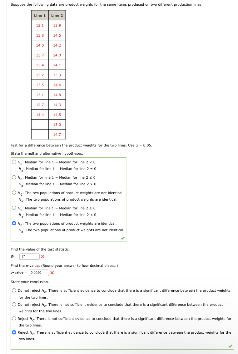
Suppose the following data are product weights for the same items produced on two different production lines. Line 1 Line 2 13.1 13.8 14.0 13.7 13.4 13.2 13.5 13.1 12.7 14.4 13.9 14.6 14.2 14.0 14.1 13.3 14.4 14.8 14.3 14.5

1) "Conservationists have despaired over destruction of tropical rain forest by logging, clearing, and burning." These words begin a report on a statistical study of the effects of logging in Borneo. Here are data on the number of tree species in 12 unlogged forest plots and 9 similar plots logged 8 years earlier: Unlogged 22 18 22 20 15 21 13 13 19 13 19 15 Logged 17 4 18 14 18 15 15 10 12 Use the data to give a 90% confidence interval for the difference in mean number of species between unlogged and logged plots. Compute degrees of freedom using the conservative method. Interval: to

Consider the following information about the payroll of NBA teams. The data is in millions of dollars. 6. 32.1 27.4 27.8 61.8 27.8 27.0 25.9 27.1 34.2 28.0 38.9 24.1 28.5 36.6 34.6 24.9 27.3 34.1 56.5 45.8 27.1 42.9 36.7 25.2 28.4 25.5 40.9 a) Make a grouped frequency distribution table with 6 classes. b) Use your table to draw a histogram. c) Circle the shape of this data. Symmetric Make a stem-and-leaf plot that makes sense. Left skewed Right skewed d)

To test for any significant difference in the number of hours between breakdowns for four machines, the following data were obtained. Machine1 Machine2 Machine3 Machine4 6.6 9.1 10.9 9.6 8.1 7.8 9.9 12.4 5.6 9.7 9.4 11.7 7.8 10.3 10.1 10.6 8.8 9.5 8.8 10.9 7.5 10.0 8.5 11.4 (a) At the ? = 0.05 level of significance, what is the difference, if any, in the population mean times among the four machines? State the null and alternative hypotheses. H0: ?1 ≠ ?2 ≠ ?3 ≠ ?4Ha: ?1 = ?2 = ?3 = ?4   H0: ?1 = ?2 = ?3 = ?4Ha: ?1 ≠ ?2 ≠ ?3 ≠ ?4       H0: At least two of the population means are equal.Ha: At least two of the population means are different.   H0: Not all the population means are equal.Ha: ?1 = ?2 = ?3 = ?4   H0: ?1 = ?2 = ?3 = ?4Ha: Not all the population means are equal.   Find the value of the test statistic. (Round your answer to two decimal places.)   Find the p-value. (Round your answer to three decimal places.) p-value =   State your conclusion. Reject…

The table below shows the number of fatal heart attacks in 19 selected European Union countries during 2014 along with the 2014 debt-to-GDP ratios for these countries in 2014. Compare the coefficients of variation and comment on your findings.   Country  Fatal Heart Attacks 2014* Debt to GDP Ratio** 1 Austria 14,521 225% 2 Belgium 7,792 327% 3 Czech Republic 26,171 128% 4 Denmark 3,943 302% 5 Finland 10,338 238% 6 France 33,513 280% 7 Germany 121,471 188% 8 Greece 12,200 317% 9 Hungary 32,138 225% 10 Ireland 4,283 390% 11 Italy 69,653 259% 12 Netherlands 8,956 325% 13 Poland 38,642 134% 14 Portugal 7,456 358% 15 Romania 50,667 104% 16 Slovakia 13,381 151% 17 Spain 32,564 313% 18 Sweden 12,617 304% 19 United Kingdom 69,325 252%

3. 4. The Global Business Travel Association reported the domestic airfare for business travel for the current year and the previous year. Below is a sample of 12 flights with their domestic airfares shown for both years. Do not round intermediate calculations. 6. Current Year Previous Year Current Year Previous Year 7. 315 576 510 534 8. 462 264 597 243 9. 276 387 282 288 432 234 648 306 10. 534 465 693 549 273 75 381 522 a. Formulate the hypotheses and test for a significant increase in the mean domestic airfare for business travel for the one-year period. Ho: Hd Select your answer - ▼ Ha Hd ·Select your answer - ▼ What is the p-value? (to 3 decimals) t-value Degrees of freedom p-value is - Select your answer - Using a 0.05 level of significance, what is your conclusion? v that there has been a significance increase in business travel. airfares over the one- We - Select your answer - year period. b. What is the sample mean domestic airfare for business travel for each year? Current…

The data below represents international sales versus Canada sales for the McDonalds's Chain. Year Canada Sales International Sales 1987 7.6 2.3 1988 7.9 2.6 1989 8.3 2.9 1990 8.6 3.2 1991 8.8 3.7 1992 9.0 4.1 1993 9.4 4.8 1994 10.2 5.7 1995 11.4 7.0 1996 12.1 8.9 Required: Regress McDonald's international sales then answer the questions: a. What is the regression model? b. Interpret your results Type your numeric answerand submit

Suppose the following table represents world oil production in millions of barrels a day for a recent period of time. Complete parts a and b. Region Oil Production​ (millions of barrels a​ day) Iran 6.97 Saudi Arabia 8.76 Other OPEC countries 21.77 ​Non-OPEC countries 53.53 Question content area bottom Part 1 a. Compute the percentage of values in each category. Region Oil Production​ (millions of barrels a​ day) Percentage Iran 6.97    enter your response here​% Saudi Arabia 8.76    enter your response here​% Other OPEC countries 21.77    enter your response here​% ​Non-OPEC countries 53.53    enter your response here​% ​(Round to two decimal places as​ needed.) Part 2 b. What conclusions can you reach concerning the production of oil in the specified time​ period? Oil production by​ non-OPEC countries accounted for ▼ less than a quarter more than half slightly less than half more than three dash quarters of total oil production. Oil production by OPEC countries other than Iran…

The following information was recorded in a toy store: Year 2016 Year 2017 Year 2018 Price Quantity Price Quantity Price Quantity Slime 6. 50 9. 60 10 56 Sticky tact 100 2 105 120 Stinky egg Teddy Bear 4 60 4 50 60 10 30 11 26 12 24 Tortoise 8 40 11 39 12 36 (a) By using the above data, compute the Laspeyres Price Index for year 2018 by using year 2016 as base year. (b) Interpret your answer in part (a)). (c) By using the above data, compute the Paasche Price Index for year 2018 by using year 2016 as base year. (d) Which item has experienced the greatest inflation rate from year 2017 to year 2018? (Just state vour answer, no calculation is needed in part (d)).

In order to determine a realistic price for a new product that a company wants to market the company’s research department selected 10 sites thought to have essentially identical sales potential and offered the product in each at a different price. The resulting sales are recorded in the accompanying table:    Price ($) Sales ($1,000s) 15.00 15 15.50 14 16.00 16 16.50 9 17.00 12 17.50 10 18.00 8 18.50 9 19.00 6 19.50 5   c). Find the equation of the sample regression line using Minitab.  d). Interpret the meaning of the coefficients of the equation of the sample regression line.