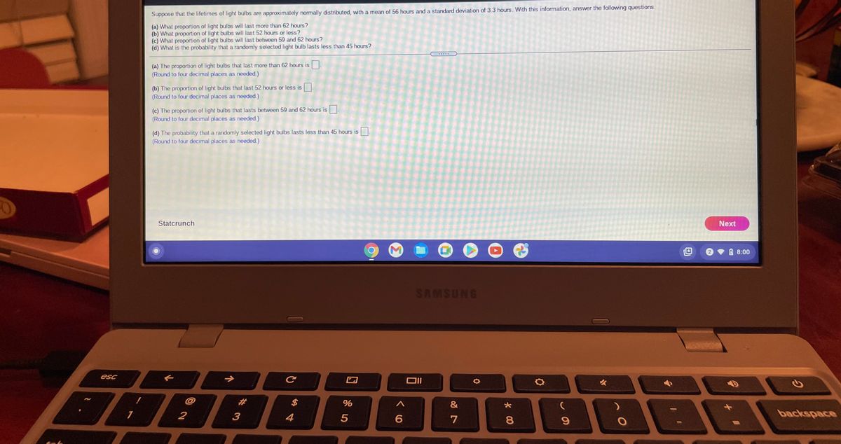
Suppose that the lifetimes of light bubs are approximately normaily dstributed, with a mean of 56 hours and a standard deviation of 3.3 hours. With this information, answer the following questions. (a) What proportion of light bubs will last more than 62 hours? (b) What proportion of light buibs will last 52 hours or less? (c) What proportion of light bulbs will last between 59 and 62 hours? (d) What is the probability that a randomly selected light bulb lasts less than 45 hours? (a) The proportion of light bulbs that last more than 62 hours is (Round to four decimal places as needed) (b) The proportion of light bubs that last 52 hours or less is (Round to four decimal places as needed.) (c) The proportion of light bulbs that lasts between 59 and 62 hours is (Round to four decimal places as needed) (d) The probablity that a randomily selected light bulbs lasts less than 45 hours is (Round to four decimal places as needed)

1) The average amount of rainfall in Puerto Rico during the past month was 3.5 inches, according to the National Meteorology Center. Suppose that a normal distribution can be used and that the standard deviation is 0.8 inches. to. What percentage of the time last month's rainfall was greater than 4 inches? b. What percentage of the time was the rainfall less than 3 inches? c. A month is considered extremely wet if the rainfall is 10% higher for that month. How much rainfall must be in April for it to be considered an extremely wet month?

The seasonal output of a new experimental strain of pepper plants was carefully weighed. The mean weight per plant is 17.0 pounds, and the standard deviation of the normally distributed weights is 1.75 pounds. Of the 200 plants in the experiment, how many produced peppers weighing between 13 and 16 pounds?

Suppose that the daily intake of an adult follows a uniform distribution from 40 to 65 micrograms. Suppose that 36 adults are randomly selected. What is the mean and standard deviation of the average intake for 36 adults. a. Mean= 52.5 stvdev = 1.2 b. Mean = 55 stvdev= 7.22c. Mean = 52.5 stvdev = 2.08 d. Mean= 52.5 stvdev = 7.22

12.) The FAA has to periodically revise their rules regarding weight estimates. Airlines use anestimate for the weight of a passenger of 195 lbs. (an adult traveling in winter including 20 lbs.of baggage). According to your textbook, assume that men (not carrying baggage) have weightsthat are normally distributed with a mean of 188.6 lbs. and a standard deviation of 38.9 lbs.a.) If one adult male is randomly selected and is assumed to be carrying 20 lbs. carry-onbaggage, find the probability that the total weight is greater than 195 lbs.b.) What total weight would separate the lower 20% of men carrying 20 lbs. of baggage fromthe top 80%?

In a mid-size company, the distribution of the number of phone calls answered each day by each of the 12 receptionists is bell-shaped and has a mean of 38 and a standard deviation of 8. Using the Standard Deviation Rule (as presented in the book), what is the approximate percentage of daily phone calls numbering between 30 and 46?

1. The fuel efficiency of a new model pick-up truck (truck) is measured in miles per gallon (mpg). A company claims that their new truck gets 25 mpg on average. A consumer group thinks the company is lying and claims that the mean mileage for all the trucks is less than 25 mpg. In a random sample, of forty-five of these trucks the mean mpg was 23.3 mpg with a standard deviation of 5.1 mpg. a. Conduct a hypothesis test to test the consumer group's claim at the 5% significance level. Be sure to state you Ho and Ha, your test statistic and p- value, whether or not you reject Ho and whether you support the claim. b. Write a complete sentence describing what a Type I error is in context. c. Write a complete sentence describing what a Type II error is in context.

The warranty on a car battery is 30 months. If the breakdown times of this battery are normally distributed with a mean of 40 months and a standard deviation of 8 ​months, determine the percent of batteries that can be expected to require repair or replacement under warranty.    what ​% of batteries can be expected to require repair or replacement under warranty.​ (Round to two decimal places as​ needed.)

1) A​ half-century ago, the mean height of women in a particular country in their 20s was 63.7 inches. Assume that the heights of today's women in their 20s are approximately normally distributed with a standard deviation of 2.31 inches. If the mean height today is the same as that of a​ half-century ago, what percentage of all samples of 26 of today's women in their 20s have mean heights of at least 65.04 ​inches?