
ENGR.ECONOMIC ANALYSIS
14th Edition
ISBN: 9780190931919
Author: NEWNAN
Publisher: Oxford University Press
expand_more
expand_more
format_list_bulleted
Related questions
Question
thumb_up100%
Given the solution for a to c. Show clear working for questions d to f
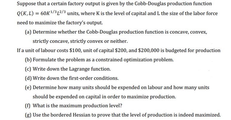

Transcribed Image Text:Suppose that a certain factory output is given by the Cobb-Douglas production function
Q(K,L) = 60K¹/312/3 units, where K is the level of capital and L the size of the labor force
need to maximize the factory's output.
(a) Determine whether the Cobb-Douglas production function is concave, convex,
strictly concave, strictly convex or neither.
If a unit of labour costs $100, unit of capital $200, and $200,000 is budgeted for production
(b) Formulate the problem as a constrained optimization problem.
(c) Write down the Lagrange function.
(d) Write down the first-order conditions.
(e) Determine how many units should be expended on labour and how many units
should be expended on capital in order to maximize production.
(f) What is the maximum production level?
(g) Use the bordered Hessian to prove that the level of production is indeed maximized.

Transcribed Image Text:4:08 AO
Expert Solution
bartleby.com/questions-and-
• Q is the output level
• K is the level of capital input
• L is the level of labor input
Step 1
The Cobb-Douglas production function is a widely used function
in economics to model the relationship between the inputs used
in production and the resulting output. It is given by the
following functional form:
Q=A* K^a* L^B
where:
• A is a productivity factor
• a and ẞ are parameters that measure the share of output
produced by each input
²01²
-40K(1/3) L(-4/3)
Ə²Q/ƏKƏL = 40 / 3k K(-2/3) L(-1/3)
=
The parameters a and ß are typically assumed to be positive and
less than one, which implies that the production function
H =
exhibits decreasing returns to scale. In other words, as the inputs
are increased proportionately, the resulting increase in output is
less than proportionate.
Step 2
(a) To determine whether the Cobb-Douglas production function
is concave, convex, strictly concave, strictly convex, or neither,
we need to compute the second-order partial derivatives of the
function.
Q(K,L) = 60K(1/3)* L(2/3)
Taking the first-order partial derivatives, we get:
?Q / ?к = 20K(-2/3)(2/3)
aQ/L = 40K(1/3) (-1/3)
Taking the second-order partial derivatives, we get:
a²Q/ Ək²
= -40K K(-5/3) (2/3)
a²Q/ ak² a² QƏKƏL
²/ KA²²
det(H) = (a²Q/ƏK²) (A²Q/ ƏL²)-(0²Q / ƏKƏL)²
ŵ
LTE+
↓↑
To determine the concavity or convexity of the function, we can
compute the determinant of the Hessian matrix:
(b) The budget constraint is:
$ 200K + $ 100L = $ 200,000
all 30%
(c) The Lagrange function is:
L(K, L, X) = 60K(1/3) (2/3)
+ >($ 200K +
+ :D
|||
det(H) = -40K
(-5/3) T
(2/3),
Substituting the second-order partial derivatives, we get:
*(-40K(¹/3) L(-4/3) - (40/3K-2/3) L(-1/3) 2 det(H) = 3200/9K(-8/3) (-10/3)
Since det(H) is always positive, the Cobb-Douglas production
function is strictly convex.
$ 100L
WAS THIS HELPFUL?
$ 200,000)
SAVE
Expert Solution
This question has been solved!
Explore an expertly crafted, step-by-step solution for a thorough understanding of key concepts.

This is a popular solution

Trending nowThis is a popular solution!

Step by stepSolved in 6 steps

Knowledge Booster


Learn more about
Need a deep-dive on the concept behind this application? Look no further. Learn more about this topic, economics and related others by exploring similar questions and additional content below.Similar questions
- Most manufacturing companies divide manufacturing costs into which three broad categories?arrow_forwardCEO of Ganymede company produces goods with 500 customers where the number of customers is equal to Q produced, with the cost function TC = 2Q2 + 400Q + 1,300,000. Questions a. Determine fixed costs, variable costs and average costs that the customer musr pay. Describe the calculations! b.If the item sells for 5,000 and 7,000, determine the position of the company and can the company grow?arrow_forward
Recommended textbooks for you
 Principles of Economics (12th Edition)EconomicsISBN:9780134078779Author:Karl E. Case, Ray C. Fair, Sharon E. OsterPublisher:PEARSON
 Engineering Economy (17th Edition)EconomicsISBN:9780134870069Author:William G. Sullivan, Elin M. Wicks, C. Patrick KoellingPublisher:PEARSON
 Principles of Economics (MindTap Course List)EconomicsISBN:9781305585126Author:N. Gregory MankiwPublisher:Cengage Learning
 Managerial Economics: A Problem Solving ApproachEconomicsISBN:9781337106665Author:Luke M. Froeb, Brian T. McCann, Michael R. Ward, Mike ShorPublisher:Cengage Learning
 Managerial Economics & Business Strategy (Mcgraw-...EconomicsISBN:9781259290619Author:Michael Baye, Jeff PrincePublisher:McGraw-Hill Education
Principles of Economics (12th Edition)
Economics
ISBN:9780134078779
Author:Karl E. Case, Ray C. Fair, Sharon E. Oster
Publisher:PEARSON
Engineering Economy (17th Edition)
Economics
ISBN:9780134870069
Author:William G. Sullivan, Elin M. Wicks, C. Patrick Koelling
Publisher:PEARSON
Principles of Economics (MindTap Course List)
Economics
ISBN:9781305585126
Author:N. Gregory Mankiw
Publisher:Cengage Learning
Managerial Economics: A Problem Solving Approach
Economics
ISBN:9781337106665
Author:Luke M. Froeb, Brian T. McCann, Michael R. Ward, Mike Shor
Publisher:Cengage Learning
Managerial Economics & Business Strategy (Mcgraw-...
Economics
ISBN:9781259290619
Author:Michael Baye, Jeff Prince
Publisher:McGraw-Hill Education