
MATLAB: An Introduction with Applications
6th Edition
ISBN: 9781119256830
Author: Amos Gilat
Publisher: John Wiley & Sons Inc
expand_more
expand_more
format_list_bulleted
Related questions
Topic Video
Question
thumb_up100%
STEP 1: State the hypotheses and select an alpha level.
H0: µ1 = µ2 = µ3 (There is no treatment effect.)
H1: At least one of the treatment means is different.
We use α = .05
STEP 2: Locate the critical region.
df total = N - 1 =
df between = k - 1 = (Numerator)
df within = N – k = (Denominator)
look up in the f table: df = Numerator, Denominator, Critical region =
STEP 3: Compute the F-ratio.
SS total = ΣX^2-G^2/N =
SS within = ΣSS inside each treatment =
SSbetween = SStotal – SSwithin
=
Calculation of
MS between=(SS between)/(ⅆf between)
MS within=(SS within)/(ⅆf within)
Calculation of F.
F=(MS between)/(MS within)
=
STEP 4 : MAKE A DECISION
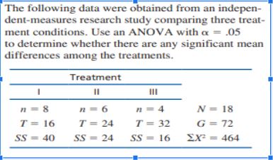

Transcribed Image Text:The following data were obtained from an indepen-
dent-measures research study comparing three treat-
ment conditions. Use an ANOVA with a = .05
to determine whether there are any significant mean
differences among the treatments.
Treatment
II
n = 8
n = 6
n = 4
N = 18
T = 16
T = 24
T = 32
G = 72
SS = 40
SS = 24
SS = 16
EX = 464
%3D

Transcribed Image Text:The F Distribution*
*Table entries in lightface type are critical values for the 05 level of significance.
Boldface type values are for the .01 level of significance.
Criticał
Degrees of
Freedom:
Denominator
Degrees of Freedom: Numerator
3.
4
7
8
9
10
11
12
14
16
20
1
239
200
4999 5403 5625
216
230
5764
161
225
234
237
241
242
243
244
246
6106 6142 6169 6208
245
248
4052
5859
5928
5981
6022
6056
6082
19.36
19.37
19.38
19.41 19.42 19.43 19.44
99.42 99.43 99.44 99.45
2
18.51 19.00 19.16 19.25 19.30 19.33
19.39
19.40
98.49 99.00 99.17 99.25 99.30 99.33
99.34
99.36 99.38
99.40 99.41
8.88
28.24 27.91 27.67
8.94
8.84
8.81
8.69 8.66
27.23 27.13 27.05 26.92 26.83 26.69
10.13 9.55 9.28
9.12
9.01
8.78
8.76
8.74
8.71
3.
34.12 30.92 29.46 28.71
27.49 27.34
6.04
5.96
14.54 14.45 14.37 14.24 14.15 14.02
6.94
6.59
6.39
6.26
6.16
6.09
6.00
5.91
5.87
7.71
21.20 18.00 16.69 15.98
4
5.93
5.84
5.80
15.52 15.21 14.98
14.80 14.66
6.61
5.79
5.19
5.05
4.95
4.88
4.82
4.78
4.74
4.70
1.68
1.61
1.60 1.56
9.68
5
5.41
16.26 13.27 12.06 11.39 10.97 10.67 10.45
10.27 10.15
10.05
9.96
9.89
9.77
9.55
4.15
8.10
5.14 4.76
4.53
4.10
4.06
4.39
8.75
4.00
7.72
6
5.99
4.28
4.21
4.03
3.96
3.92 3.87
13.74 10.92 9.78
9.15
8.47
8.26
7.98
7.87
7.79
7.60
7.52
7.39
3.79
3.73
6.84
4.74 4.35
3.97
3.87
3.68
3.63
3.60
5.59
12.25
3.49
6.27
7
4.12
3.57
3.52
3.44
9.55 8.45
7.85
7.46
7.19
7.00
6.71
6.62
6.54
6.47
6.35
6.15
3.50
6.19
3.28
5.67
4.46 4.07
3.69
3.58
6.37
3.39
5.91
3.34
3.31
3.23
5.56
5.32
3.84
3.44
3.20
5.48
3.15
5.36
8
11.26
8.65 7.59
7.01
6.63
6.03
5.82
5.74
5.12
3.37
3.23
3.29.
5.62
3.18
3.13
3.10
3.07
5.11
4.26 3.86
3.02
3.63
6.42
9.
3.48
2.98
2.93
10.56
8.02 6.99
6.06
5.80
5.47
5.35
5.26
5.18
5.00
4.92
4.80
3.07
5.06
2.97
3.02
4.95
2.91
4.71
2.94
4.96
10.04
3.48
3.33
5.64
3.22
3.14
5.21
2.86
4.60
4.10 3.71
2.82
4.52
10
2.77
7.56 6.55
5.99
5.39
4.85
4.78
4.41
3.09
5.07
2.95
2.90
4.84
9.65
3.59
6.22
3.20
5.32
2.82
4.46
I 1
3.98
3.36
3.01
2.86
2.79
2.74
2.70 2.65
7.20
5.67
4.88
4.74
4.63
4.54
4.40
4.29
4,21
4.10
3.26
5.41
3.00
4.82
2.80
4.39
2.76
4.30
3.49
2.69
3.11
5.06
2.92
2.85
4.50
2.72
4.22
2.64
2.60 2.54
4.75
9.33
3.88
6.93 5.95
12
4.65
4.16
4.05
3.98
3.86
2.67
4.10
2.63
3.02
4.86
2.92
2.84
2.77
2.72
2.60
4.67
9.07
3.80
6.70 5.74
2.55
3.85
3.18
2.51
3.78
13
3.41
2.46
5.20
4.62
4.44
4.30
4.19
4.02
3.96
3.67
2.85
2.65
4.03
14
4.60
3.74
3.34
3.11
2.96
2.77
2.70
2.60
2.56
2.53
2.48
2.44
2.39
8.86
6.51
5.56
5.03
4.69
4.46
4.28
4.14
3.94
3.86
3.80
3.70
3.62 3.51
2.79
2.59
2.55
2.70
4.14
2.64
2.48
2.43
2.39
3.56 3.48
2.90
2.51
2.33
4.54
8.68
15
3.68
3.29
3.06
6.36
5.42
4.89
4.56
4.32
4.00
3.89
3.80
3.73
3.67
3.36
2.66
2.59
3.89
2.54
2.8.5
4.44
2.74
2.49
2.45
2.42
2.37
2.28
3.37 3.25
16
4.49
3.63
3.24
3.01
2.33
8.53
6.23
5.29
4.77
4.20
4.03
3.78
3.69
3.61
3.55
3.45
Expert Solution
This question has been solved!
Explore an expertly crafted, step-by-step solution for a thorough understanding of key concepts.

Step by stepSolved in 2 steps

Knowledge Booster


Learn more about
Need a deep-dive on the concept behind this application? Look no further. Learn more about this topic, statistics and related others by exploring similar questions and additional content below.Similar questions
- Comment on the P-value for testing the claim μ1- μ2=0arrow_forwardA test of H0: µ ≥ 59 versus H1: µ < 59 is performed using α = 0.05. The value of the test statistic z = -1.80. If the true value of µ is 59, does the conclusion you reach result in Type I error, Type II error, or the correct decision? a. Type I Error b. Type II Error c. correct decision d. not enough informationarrow_forwardYou run a regression analysis on a bivariate set of data (n=82n=82). You obtain the regression equationy=4.373x+9.596y=4.373x+9.596with a correlation coefficient of r=0.987r=0.987 (which is significant at α=0.01α=0.01). You want to predict what value (on average) for the explanatory variable will give you a value of 60 on the response variable.What is the predicted explanatory value?x = (Report answer accurate to one decimal place.)arrow_forward
- Preliminary data analysis indicate that it is reasonable to use a t-test to carry out the specified hypothesis test. Perform the t-test using the critical-value approach. %3D X = 44.2 and s = 7.3 Use a significance level of a = 0.05 to test the claim that u 35.8. The sample data consists of 10 scores for which H:µ±35.8 0 Н и-35.8 Test statistics: t=3.64 Critical Value: t=+/-2.262 H:µ=35.8 Reject There is sufficient evidence to support the claim that the mean is different from 35.8. П. : и 3 44.2 0. H:µ±44.2 a. Test statistics: t=3.64 Critical Value: t= +/- 2.262 H:µ=44.2 Н, There is sufficient evidence to support the claim that the mean is different from 44.2. Rejectarrow_forwardChildhood participation in sports, cultural groups, and youth groups appears to be related to improved self-esteem for adolescents (McGee, Williams, Howden-Chapman, Martin, & Kawachi, 2006). In a representative study, a sample of n = 100 adolescents with a history of group participation is given a stan- dardized self-esteem questionnaire. For the general population of adolescents, scores on this questionnaire form a normal distribution with a mean of p %3D 50 and %3D 15. The sample of group- a standard deviation of o %3D participation adolescents had an average of M = 53.8.arrow_forwardYou run a regression analysis on a bivariate set of data (n=19n=19). You obtain the regression equationy=1.761x+1.382y=1.761x+1.382with a correlation coefficient of r=0.876r=0.876 (which is significant at α=0.01α=0.01). You want to predict what value (on average) for the explanatory variable will give you a value of 160 on the response variable.What is the predicted explanatory value?x = (Report answer accurate to one decimal place.)arrow_forward
- al Exam tps://ezto.mher nework: Chapte ections 84 O You received partial credit in the previous attempt. Check my work View previous attempt Concerns about climate change and CO2 reduction have initiated the commercial production of blends of biodiesel (e.g., from renewable sources) and petrodiesel (from fossil fuel). Random samples of 41 blended fuels are tested in a lab to ascertain the bio/total carbon ratio. (a) If the true mean is .9220 with a standard deviation of 0.0060, within what interval will 90 percent of the sample means fall? (Round your answers to 4 decimal places.) The interval is from Ito (b) If the true mean is .9220 with a standard deviation of 0.0060, what is the sampling distribution of X ? 1. Exactly normal with u=.9220 and o = 0.0060. 2. Approximately normal with µ = .9220 and o = 0.0060. 3. Exactly normal with u=.9220 and o = 0.0060 /41 4. Approximately normal with µ= .9220 and o = 0.0060 //41. Retake Use Photoarrow_forwardplease show all steps USING EXCEL ONLY FORMULASarrow_forwardWhat can you conclude? show step by step procedure using BOTH p-value and critical region Explain solution in the most simple practical terms The carbon monoxide (CO) level in a manufacturing plant is supposed to be about 50 parts per million (ppm). However the actual CO levels are quite variable. Five CO measurements are taken at various times during the day: 58 63 48 52 68 a. Test if the CO levels are equal to 50ppm vs not equal to 50ppmarrow_forward
arrow_back_ios
arrow_forward_ios
Recommended textbooks for you
- MATLAB: An Introduction with ApplicationsStatisticsISBN:9781119256830Author:Amos GilatPublisher:John Wiley & Sons Inc
 Probability and Statistics for Engineering and th...StatisticsISBN:9781305251809Author:Jay L. DevorePublisher:Cengage Learning
 Statistics for The Behavioral Sciences (MindTap C...StatisticsISBN:9781305504912Author:Frederick J Gravetter, Larry B. WallnauPublisher:Cengage Learning
  Elementary Statistics: Picturing the World (7th E...StatisticsISBN:9780134683416Author:Ron Larson, Betsy FarberPublisher:PEARSON
 The Basic Practice of StatisticsStatisticsISBN:9781319042578Author:David S. Moore, William I. Notz, Michael A. FlignerPublisher:W. H. Freeman
 Introduction to the Practice of StatisticsStatisticsISBN:9781319013387Author:David S. Moore, George P. McCabe, Bruce A. CraigPublisher:W. H. Freeman
MATLAB: An Introduction with Applications
Statistics
ISBN:9781119256830
Author:Amos Gilat
Publisher:John Wiley & Sons Inc
Probability and Statistics for Engineering and th...
Statistics
ISBN:9781305251809
Author:Jay L. Devore
Publisher:Cengage Learning
Statistics for The Behavioral Sciences (MindTap C...
Statistics
ISBN:9781305504912
Author:Frederick J Gravetter, Larry B. Wallnau
Publisher:Cengage Learning
Elementary Statistics: Picturing the World (7th E...
Statistics
ISBN:9780134683416
Author:Ron Larson, Betsy Farber
Publisher:PEARSON
The Basic Practice of Statistics
Statistics
ISBN:9781319042578
Author:David S. Moore, William I. Notz, Michael A. Fligner
Publisher:W. H. Freeman
Introduction to the Practice of Statistics
Statistics
ISBN:9781319013387
Author:David S. Moore, George P. McCabe, Bruce A. Craig
Publisher:W. H. Freeman