
MATLAB: An Introduction with Applications
6th Edition
ISBN: 9781119256830
Author: Amos Gilat
Publisher: John Wiley & Sons Inc
expand_more
expand_more
format_list_bulleted
Related questions
Question
Q4. In simulation study of a manufacturing system, both the average daily production rates obtained from simulation model (use data from day n1/2 to day n2/2, round it to nearest integer) and from the real system are given, in data set 3.
- n1= 27.6. n2=97.6
- Apply t test to decide if we can assume the simulation model is a valid representation of the real system is given.
- Check if we can assume the average daily production rates obtained from simulation in successive days are independent by using scatter diagram (X Y plot in excel; X axis Xi value Y axis Xi+1)
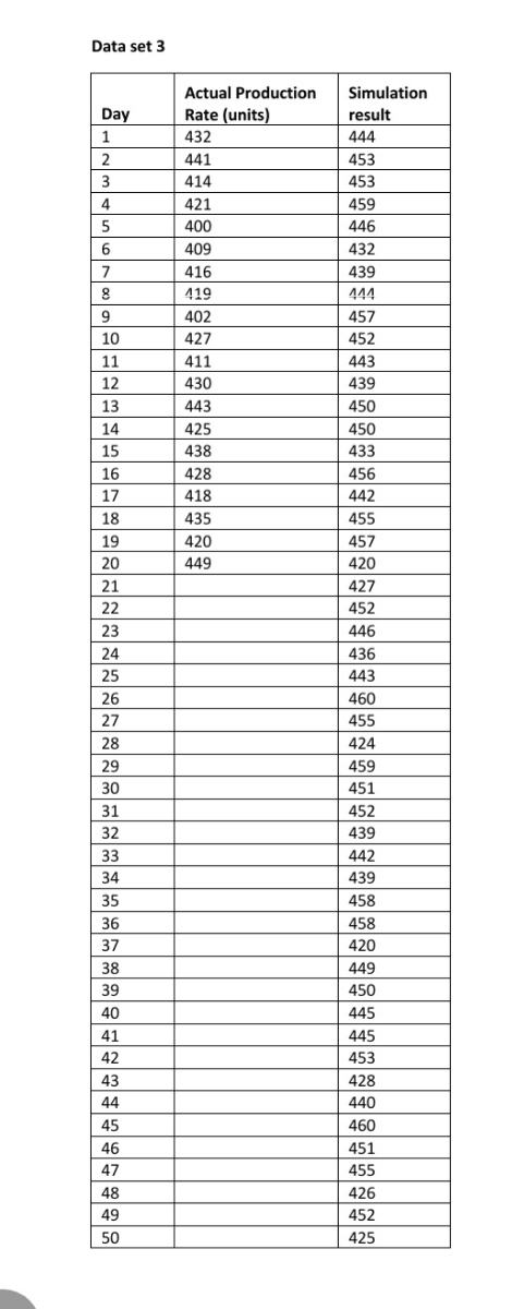

Transcribed Image Text:Data set 3
Day
1
2
3
4
5
6
7
8
9
10
11
12
13
14
15
16
17
18
19
20
21
22
23
24
25
26
27
28
29
30
31
32
33
34
35
36
37
38
39
40
41
42
43
44
45
46
47
48
49
50
Actual Production
Rate (units)
432
441
414
421
400
409
416
419
402
427
411
430
443
425
438
428
418
435
420
449
Simulation
result
444
453
453
459
446
432
439
444
457
452
443
439
450
450
433
456
442
455
457
420
427
452
446
436
443
460
455
424
459
451
452
439
442
439
458
458
420
449
450
445
445
453
428
440
460
451
455
426
452
425
Expert Solution
arrow_forward
Step 1
Given information:
Consider the given dataset:
| Actual Production Rate | Simulation Result |
| 432 | 444 |
| 441 | 453 |
| 414 | 453 |
| 421 | 459 |
| 400 | 446 |
| 409 | 432 |
| 416 | 439 |
| 419 | 444 |
| 402 | 457 |
| 427 | 452 |
| 411 | 443 |
| 430 | 439 |
| 443 | 450 |
| 425 | 450 |
| 438 | 433 |
| 428 | 456 |
| 418 | 442 |
| 435 | 455 |
| 420 | 457 |
| 449 | 420 |
| 427 | |
| 452 | |
| 446 | |
| 436 | |
| 443 | |
| 460 | |
| 455 | |
| 424 | |
| 459 | |
| 451 | |
| 452 | |
| 439 | |
| 442 | |
| 439 | |
| 458 | |
| 458 | |
| 420 | |
| 449 | |
| 450 | |
| 445 | |
| 453 | |
| 428 | |
| 440 | |
| 460 | |
| 451 | |
| 455 | |
| 426 | |
| 452 | |
| 425 |

Step by stepSolved in 3 steps with 4 images

Knowledge Booster

Similar questions
- 1.)fill in the blanks. Based on the physician's study, the predictor variable, X is_____and the response variable, Y, is________. 2.) As described in the article, the relation between age and peak heart is a______. - positive relation - negative relation - no relation 3.) Provide the regression line, ŷ=a+bx. Show steps/equations used to get answer. 4.) Suppose a 40 year old person is randomely selected. Use your Model to predict their peak heart rate. 5.) Based on your model, as a person ages one year, how much would you expect peak heart rate to change?arrow_forwardplz solve question (c) with explanation within 30-40 mins and get upvotesarrow_forwardz score z score for each for each value of value of Zzły х х -0.278 0.536 -0.149 -0.089 0.696 -0.062 -1.253 -1 -1.652 2.070 -0.714 -0.928 0.663 2.461 1.473 1.671 0.536 0.371 0.199 -0.089 4 -0.278 0.025 Σ: ỹ = 3.857 S, = 3.078 = 5.207 T= 4.286 s, = 3.200arrow_forward
- Below is my script for some problems I am doing in RStudio. How do I code to get the statistical data that shows how the male tv hours differ to the female tv hours? Chapter 2 R Lab.R X StudentSurvey.(1) x Source on SaveE T # 3- Ine Exercise nours are skewea Tert 8 xtabs (~Year, Student Survey. (1)) 9 # 1- The highest concentration of students are Sophomores 10 table(Year)/length (Year) II # 2- The relative frequency for seniors was 0.1% (rounded) 11 Student Survey. (1) STV 12 12 TV 13 14 23 15 16 29 18 19 20 21 22 23 21 24:1 hist (TV) →→Run boxplot (TV) # 6- Based on the box plot there is not a smallest outlier, but there are large outliers # The outliers for hours spent watching TV are any values above 20 hours Survey - Student Survey. (1) #Renaming xtabs (~Sex, Survey) install.packages ("lattice") library("lattice") bwplot (TV Sex, Survey) # 7- Men on average watch more TV # 8- Men have more variability in hours watching TV (Top Level) + Source R Script =arrow_forwardI need help with this assaigmentarrow_forwardHelp me pleasearrow_forward
arrow_back_ios
arrow_forward_ios
Recommended textbooks for you
- MATLAB: An Introduction with ApplicationsStatisticsISBN:9781119256830Author:Amos GilatPublisher:John Wiley & Sons Inc
 Probability and Statistics for Engineering and th...StatisticsISBN:9781305251809Author:Jay L. DevorePublisher:Cengage Learning
 Statistics for The Behavioral Sciences (MindTap C...StatisticsISBN:9781305504912Author:Frederick J Gravetter, Larry B. WallnauPublisher:Cengage Learning
  Elementary Statistics: Picturing the World (7th E...StatisticsISBN:9780134683416Author:Ron Larson, Betsy FarberPublisher:PEARSON
 The Basic Practice of StatisticsStatisticsISBN:9781319042578Author:David S. Moore, William I. Notz, Michael A. FlignerPublisher:W. H. Freeman
 Introduction to the Practice of StatisticsStatisticsISBN:9781319013387Author:David S. Moore, George P. McCabe, Bruce A. CraigPublisher:W. H. Freeman
MATLAB: An Introduction with Applications
Statistics
ISBN:9781119256830
Author:Amos Gilat
Publisher:John Wiley & Sons Inc
Probability and Statistics for Engineering and th...
Statistics
ISBN:9781305251809
Author:Jay L. Devore
Publisher:Cengage Learning
Statistics for The Behavioral Sciences (MindTap C...
Statistics
ISBN:9781305504912
Author:Frederick J Gravetter, Larry B. Wallnau
Publisher:Cengage Learning
Elementary Statistics: Picturing the World (7th E...
Statistics
ISBN:9780134683416
Author:Ron Larson, Betsy Farber
Publisher:PEARSON
The Basic Practice of Statistics
Statistics
ISBN:9781319042578
Author:David S. Moore, William I. Notz, Michael A. Fligner
Publisher:W. H. Freeman
Introduction to the Practice of Statistics
Statistics
ISBN:9781319013387
Author:David S. Moore, George P. McCabe, Bruce A. Craig
Publisher:W. H. Freeman