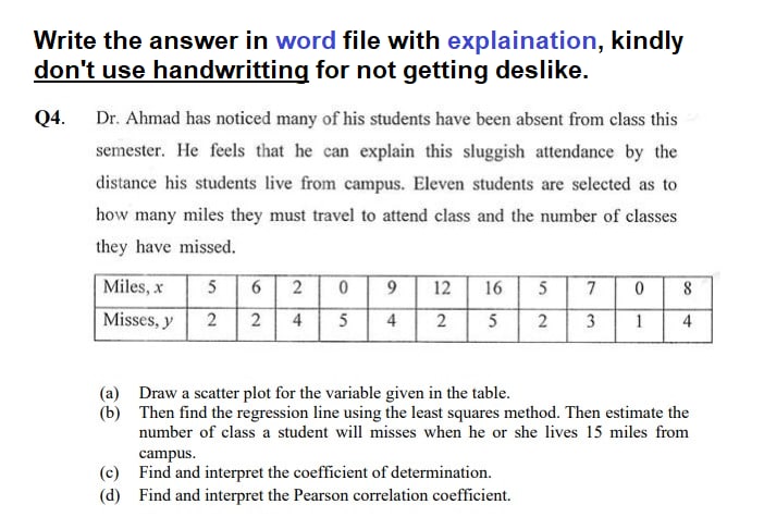
Q4. Dr. Ahmad has noticed many of his students have been absent from class this semester. He feels that he can explain this sluggish attendance by the distance his students live from campus. Eleven students are selected as to how many miles they must travel to attend class and the number of classes they have missed. Miles, x 5 6 2 0 9 12 5 7 0 8 Misses, y 2 2 4 5 4 2 2 3 1 4 (a) Draw a scatter plot for the variable given in the table. (b) Then find the regression line using the least squares method. Then estimate the number of class a student will misses when he or she lives 15 miles from campus. (c) Find and interpret the coefficient of determination. Find and interpret the Pearson correlation coefficient. (d) 25 16

please show thanks

a) Find the equation of the line which is the best fit for the data, with x equal to the number of years after 1999 and y equal to the millions of people b) Ise the model to estimate the number of people who took trips in 2008.

The table and scatter plot show the number of years of experience, x, and the hourly pay rate, y, for each of 10 cashiers in Arizona. The equation of the line of best fit is y = 0.9xr+8.22. Experience, x Hourly pay rate, y (in years) 22 (in dollars) 20+ 0.8 7.47 18- 1.1 9.46 +16- Hourly 2.2 8.91 14+ pay rate 3.1 11.46 (in dollars) 124 10 3.8 12.31 3.8 13.00 6- 5.0 14.50 6.9 12.40 8.5 15.44 10 10 11 8.8 15.79 Experience (in years) Use the equation of the line of best fit to fill in the blanks below. Give exact answers, not rounded approximations. Observed hourly pay Predicted hourly pay Number of years Residual (in dollars) rate rate of experience (in dollars) (in dollars) 5.0 6.9

#6. Basic Computation: Five-Number Summary, Interquartile Range 2 5 5 6 7 8 8 9 10 12 (a) Find the low, Q1, Median, Q3, and High. (b) Find the interquartile range (c) Make a box-and-whisker plot.

The table and scatter plot show the time spent studying, x, and the midterm score, y, for each of 10 students. The equation of the line of best fit is y = 3.7x+ 14.64. Time spent Midterm studying, x (in hours) 100- score, y 90 3.3 22.41 70- 3.8 30.97 Midterm score 60 4.6 25.31 50 5.9 37.96 40 6.9 36.86 30 20 8.1 53.20 10- 8.5 44.64 9.2 57.51 10 12 14 16 18 20 22 24 16 12.0 59.04 Time spent studying (in hours) 15.0 65.00 Use the equation of the line of best fit to fill in the blanks below. Give exact answers, not rounded approximations. Time spent studying (in hours) Observed midterm Predicted midterm Residual Score Score 12.0 15.0 OIO

An office supply company services copiers and tracks how many machines are serviced and the length of time (in minutes) for a service call. The data below for 11 clients is below.   Sum X = 46   Sum Y= 234  Sum XY = 5797       Sum X2 =1180         Sum Y2 =146608     1) Calculate SSYY, SSXX, SSXY   2) Calculate b0, b1   3) Interpret the estimated slope coefficient.

Homework Q1: Implement All plot types using MS Excel and Send the files Q2: What type of plot is most suitable to address the electromagnetic spectrum and why? Report Write a report about using plots for manufacturing of One of these types • • Lasers Light Emitting Diodes • Optical Switches 22

Suppose a researcher collects data on the air pollution levels, measured in milligrams per cubic meter, for both urban and rural areas in 35 states. The data is plotted with urban air pollution levels on the horizontal axis and rural air pollution levels on the vertical axis. Nevada is an outlier in the ?x‑direction. What must be true about this state? The urban air pollution levels for this state are much higher or lower than the rest of the states in the data set. The rural air pollution levels for this state are much higher or much lower than the rest of the states in the data set. This state is an influential observation. The rural air pollution levels for this state are much higher or lower than other states in the data set that have similar urban air pollution levels. The absolute value of the residual of this state is large.