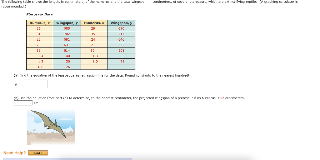
The following table shows the length, in centimeters, of the humerus and the total wingspan, in centimeters, of several pterosaurs, which are extinct flying reptiles. (A graphing calculator isrecommended.)Pterosaur DataHumerus, xWingspan, yHumerus, XWingspan, y266852969031702357172568124646236312162219614165081.4401.3331.2301.0280.826(a) Find the equation of the least-squares regression line for the data. Round constants to the nearest hundredth.(b) Use the equation from part (a) to determine, to the nearest centimeter, the projected wingspan of a pterosaur if its humerus is 52 centimeters.cmNeed Help?Read It

Given : Humerus , x Wingspan , y 26 685 31 702 25 681 23 631 19 614 1.4 40 1.2 30…

Answered: Pterosaur Data Humerus, x 26 31 25 23…

MATLAB: An Introduction with Applications

6th Edition

ISBN:9781119256830

Author:Amos Gilat

Publisher:Amos Gilat

Chapter1: Starting With Matlab

Section: Chapter Questions

Problem 1P

See similar textbooks

Similar questions

A certain town is located approximately 25 miles east of a large city. The data organized below include the appraised value (in thousands of dollars), land area of the property in acres, and age, in years, for a sample of 20 single-family homes located in the town. Develop a multiple linear regression model to predict appraised value based on land area of the property and age, in years. Complete part (a) a) State the multiple regression equation. Let X1i represent the land area of the property in acres and let X2i age, in years.
Qg- For the following data: x, 1 2 3 4 5 7 8 13 14 17 18 19 19 20 a- Find the least square regression model. b- Calculate error for x = 7 c- Estimate the correlation coefficient. Comment your result.
Find the equation of the least-squares regression line ŷ and the linear correlation coefficient r for the given data. Round the constants, a, b, and r, to the nearest hundredth. {(1, 4.5), (2, 6.0), (4, 8.4), (6, 11.7), (8, 16.2)} ŷ = r =
The table below shows the wind speed y (in mph) of a hurricane versus the barometric pressure x (in mb). of Barometric Pressure (mb) (x) Wind Speed (mph) (y) 1,005 35 1,004 45 1,000 50 996 65 984 80 970 100 949 110 929 145 904 160 a. Use the data in the table to find the least-squares regression line. Round the slope to 2 decimal places and the y-intercept to nearest whole unit. b. Use the model in part (a) to approximate the wind speed of a hurricane with a barometrie pressure of 900 mb. Select one: O a. a. y = -1.38x + 1.395: b. 153 mph Ob. a. y= -1.2x + 1.251: b. 155 mph Oc a. y= -1.2x + 1,251: b. 171 mph Od a. y=-1.38x + 1,395, b. 155 mph
Write out the regression equation based on the output.
Find the equation of the regression line for the given data. Then construct a scatter plot of the data and draw the regression line. (The pair of variables have a significant correlation.) Then use the regression equation to predict the value of y for each of the given x-values, if meaningful. The table below shows the heights (in feet) and the number of stories of six notable buildings in a city. height 775 619 519 508 491 474 (a) x=503 feet (b) x=644 feet Stories, y 53 47 44 42 39 38 (c) x=798 feet (d) x=734 feet
Biochemical oxygen demand (BOD) measures organic pollutants in water by measuring the amount of oxygen consumed by microorganisms that break down these compounds. BOD is hard to measure accurately. Total organic carbon (TOC) is easy to measure, so it is common to measure TOC and use regression to predict BOD. A typical regression equation for water entering a municipal treatment plant is BOD = -55.47 + 1.505 TOC Both BOD and TOC are measured in milligrams per liter of water. (a) What does the slope of this line say about the relationship between BOD and TOC? TOC rises (falls) by 1.505 mg/l for every 55.47 mg/l increase (decrease) in BOD BOD rises (falls) by 55.47 mg/l for every 1 mg/l increase (decrease) in TOC TOC rises (falls) by 1.505 mg/l for every 1 mg/l increase (decrease) in BOD BOD rises (falls) by 1.505 mg/l for every 1 mg/l increase (decrease) in TOC
Length, x Girth, y 136 107 168 131 151 117 145 106 159 125 160 120 123 103 138 103 156 119 147 109 146 108 145 110
I need help to interpret the slope of the scatter plot and to do the linear regression equation
In baseball, two statistics, the ERA (Earned Run Average) and the WHIP (Walks and Hits per Inning Pitched), are used to measure the quality of pitchers. For both measures, smaller values indicate higher quality. The following computer output gives the results from predicting ERA by using WHIP in a least-squares regression for the 2017 baseball season. Variable DF Estimate SE T Intercept 1 -5.0 0.26 - 19.3 WHIP 1 6.8 0.14 47.4 Which of the following statements is the best interpretation of the value 6.8 shown in the output? ERA is predicted to increase by 6.8 units for each 1 unit increase of WHIP. WHIP is predicted to increase by 6.8 units for each 1 unit increase of ERA. For a pitcher with 0 units of WHIP, the ERA is predicted to be approximately 6.8 units. For a pitcher with 0 units of ERA, the WHIP is predicted to be approximately 6.8 units. Approximately 6.8% of the variability in ERA is due to its linear relationship with WHIP.
A scatter plot shows the relationship between two quantitative variables. Each of the six scatter plots pictured shows the least-squares regression line for the corresponding data set. Classify each scatter plot according to whether the least-squares regression line has a meaningful ?y-intercept value.
Height, x 772 628 518 508 496 483 stories, y 51 48 44 43 37 35 Find the equation of the regression line for the given data. Then construct a scatter plot of the data and draw the regression line. (The pair of variables have a significant correlation.) Then use the regression equation to predict the value of y for each of the given x-values, if meaningful. The table below shows the heights (in feet) and the number of stories of six notable buildings in a city. (a) x = 498 feet (b) x = 640 feet (c) x = 345 feet (d) 735 feet Find the regression equation.Now construct a scatter plot of the data and draw the regression line. (a) Now use the regression equation to predict the value of y for each of the given x-values, if meaningful. Because the correlation between x and y is significant, the equation of the regression line can be used to predict y-values. However, prediction values are meaningful only for x-values in the range of the data. Begin with x = 498. Since x = 498…

SEE MORE QUESTIONS

Recommended textbooks for you

MATLAB: An Introduction with Applications

Statistics

ISBN:

9781119256830

Author:

Amos Gilat

Publisher:

John Wiley & Sons Inc

Probability and Statistics for Engineering and th…

Statistics

ISBN:

9781305251809

Author:

Jay L. Devore

Publisher:

Cengage Learning

Statistics for The Behavioral Sciences (MindTap C…

Statistics

ISBN:

9781305504912

Author:

Frederick J Gravetter, Larry B. Wallnau

Publisher:

Cengage Learning

MATLAB: An Introduction with Applications

Statistics

ISBN:

9781119256830

Author:

Amos Gilat

Publisher:

John Wiley & Sons Inc

Probability and Statistics for Engineering and th…

Statistics

ISBN:

9781305251809

Author:

Jay L. Devore

Publisher:

Cengage Learning

Statistics for The Behavioral Sciences (MindTap C…

Statistics

ISBN:

9781305504912

Author:

Frederick J Gravetter, Larry B. Wallnau

Publisher:

Cengage Learning

Elementary Statistics: Picturing the World (7th E…

Statistics

ISBN:

9780134683416

Author:

Ron Larson, Betsy Farber

Publisher:

PEARSON

The Basic Practice of Statistics

Statistics

ISBN:

9781319042578

Author:

David S. Moore, William I. Notz, Michael A. Fligner

Publisher:

W. H. Freeman

Introduction to the Practice of Statistics

Statistics

ISBN:

9781319013387

Author:

David S. Moore, George P. McCabe, Bruce A. Craig

Publisher:

W. H. Freeman

SEE MORE TEXTBOOKS