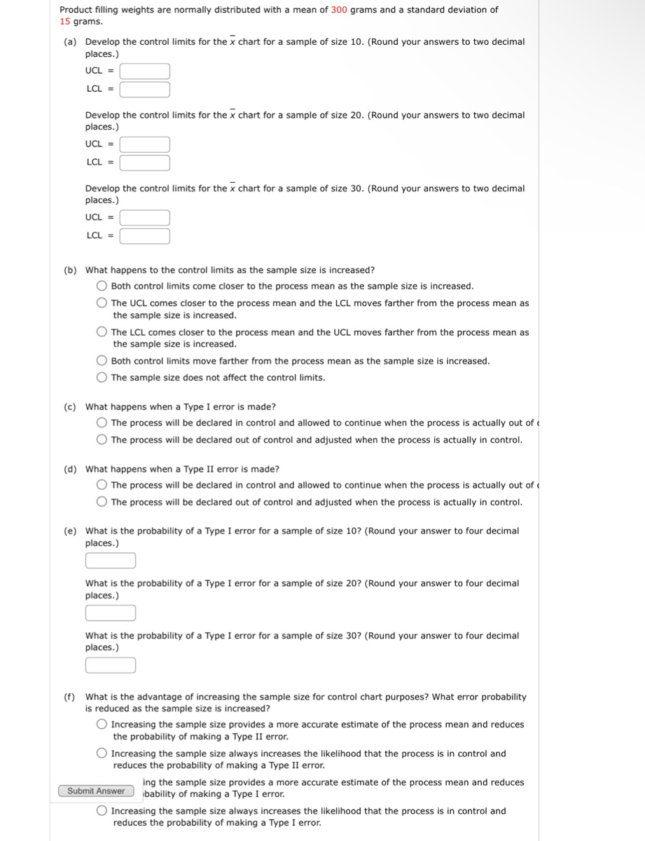
Product filling weights are normally distributed with a mean of 300 grams and a standard deviation of 15 grams. (a) Develop the control limits for the x chart for a sample of size 10. (Round your answers to two decimal places.) UCL = LCL = Develop the control limits for the x chart for a sample of size 20. (Round your answers to two decimal places.) UCL = LCL = Develop the control limits for the x chart for a sample of size 30. (Round your answers to two decimal places.) UCL = LCL= (b) What happens to the control limits as the sample size is increased? Both control limits come closer to the process mean as the sample size is increased. The UCL comes closer to the process mean and the LCL moves farther from the process mean as the sample size is increased. The LCL comes closer to the process mean and the UCL moves farther from the process mean as the sample size is increased. Both control limits move farther from the process mean as the sample size is increased. The sample size does not affect the control limits. (c) What happens when a Type I error is made? The process will be declared in control and allowed to continue when the process is actually out of The process will be declared out of control and adjusted when the process is actually in control. (d) What happens when a Type II error is made? The process will be declared in control and allowed to continue when the process is actually out of The process will be declared out of control and adjusted when the process is actually in control. (e) What is the probability of a Type I error for a sample of size 10? (Round your answer to four decimal places.) What is the probability of a Type I error for a sample of size 20? (Round your answer to four decimal places.) What is the probability of a Type I error for a sample of size 30? (Round your answer to four decimal places.) (f) What is the advantage of increasing the sample size for control chart purposes? What error probability is reduced as the sample size is increased? Increasing the sample size provides a more accurate estimate of the process mean and reduces the probability of making a Type II error. Increasing the sample size always increases the likelihood that the process is in control and reduces the probability of making a Type II error. Submit Answer ing the sample size provides a more accurate estimate of the process mean and reduces bability of making a Type I error. Increasing the sample size always increases the likelihood that the process is in control and reduces the probability of making a Type I error.

To determine if their 0.33 centimeter bolts are properly adjusted, Harper Manufacturing has decided to use an x‾-Chart which uses the range to estimate the variability in the sample. Average value 0.370 Step 1 of 7:  What is the Center Line of the control chart? Round your answer to three decimal places.   Step 2 of 7:  What is the Upper Control Limit? Round your answer to three decimal places. Step 3 of 7:  What is the Lower Control Limit? Round your answer to three decimal places.     Step 4 of 7:  Use the following sample data, taken from the next time period, to determine if the process is "In Control" or "Out of Control".Observations: 0.38,0.31,0.36,0.31,0.36,0.370.38,0.31,0.36,0.31,0.36,0.37Sample Mean: 0.34830.3483       Step 5 of 7:  Use the following sample data, taken from the next time period, to determine if the process is "In Control" or "Out of Control".Observations:…

Rachael got a 660 on the analytical portion of the Graduate Record Exam (GRE). If GRE scores are normally distributed and have mean μ = 600 and standard deviation σ = 30, what is her standardized score?

To determine if their 14 oz filling machine is properly adjusted, Harvey Soft Drinks has decided to use an X-Chart which uses the range to estimate the variability in the sample. J. Answer How to enter your answ Table Step 1 of 7: What is the Center Line of the control chart? Round your answer to three decimal places. Control Chart Period 1 2 3 4 5 6 7 8 9 10 11 Select the Copy Table button to copy all values. To select an entire row or column, either click on the row or column header or use the Shift and arrow keys. To find the average of the selected cells, select the Average Values button. Copy Table Average Values The average of the selected cell(s) is 14.000. Copy Value Sample Mean Sample Range 14.0060 0.04 0.04 0.04 0.10 0.08 0.09 0.07 0.05 0.05 0.06 0.07 obs1 obs2 obs3 obs4 obs5 14.00 13.99 14.03 14.01 14.00 14.02 14.05 14.05 14.01 14.04 14.0340 14.02 14.01 14.05 14.04 14.02 14.0280 14.04 13.97 14.05 13.95 14.00 14.0020 13.96 14.01 14.00 14.04 14.02 14.0060 13.96 14.00 14.00…