
MATLAB: An Introduction with Applications
6th Edition
ISBN: 9781119256830
Author: Amos Gilat
Publisher: John Wiley & Sons Inc
expand_more
expand_more
format_list_bulleted
Related questions
Question
Data Management - Statistical Anaylsis
Per the following graph, explain the reason for every statistic that is calculated.
For example, You have a
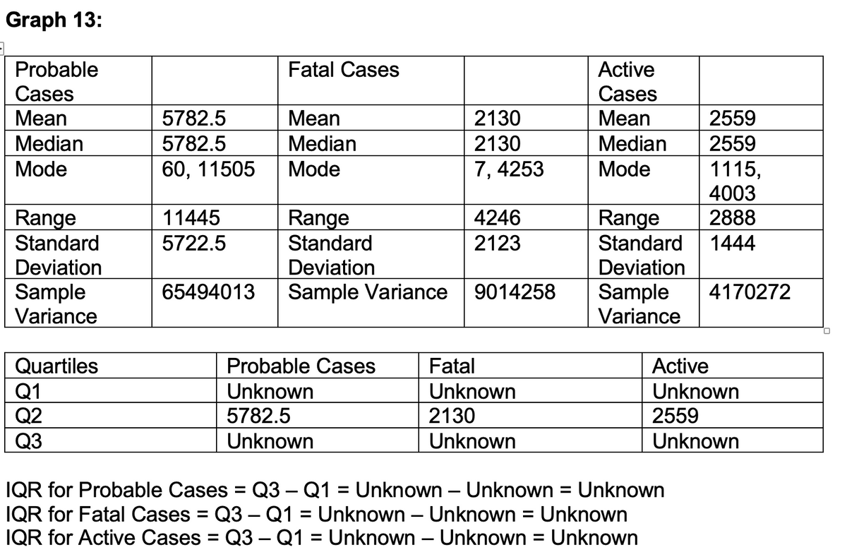

Transcribed Image Text:Graph 13:
Probable
Fatal Cases
Cases
Mean
5782.5
Mean
2130
Median
5782.5
Median
2130
Mode
60, 11505
Mode
7, 4253
Range
11445
Range
4246
Standard
5722.5
Standard
2123
Deviation
Deviation
Sample
65494013 Sample Variance 9014258
Variance
Quartiles
Probable Cases
Fatal
Q1
Unknown
Unknown
Q2
5782.5
2130
Q3
Unknown
Unknown
IQR for Probable Cases = Q3 - Q1 = Unknown - Unknown = Unknown
IQR for Fatal Cases = Q3 – Q1 = Unknown - Unknown = Unknown
IQR for Active Cases = Q3 – Q1 = Unknown - Unknown = Unknown
Active
Cases
Mean
Median
Mode
Range
Standard
Deviation
Sample
Variance
2559
2559
1115,
4003
2888
1444
4170272
Active
Unknown
2559
Unknown

Transcribed Image Text:14000
12000
10000
8000
6000
4000
2000
0
Number of Probable, Fatal, and Active Covid Cases
Fatal Cases
Probable Cases
Newly Reported
Cumulative Count
Active Cases
Expert Solution
This question has been solved!
Explore an expertly crafted, step-by-step solution for a thorough understanding of key concepts.

Step by stepSolved in 2 steps

Knowledge Booster

Similar questions
- Data Management - Statistical Anaylsis Per the following graph, explain the reason for every statistic that is calculated. For example, You have a scatter plot of an hourly wages vs level of education, the trend is represented by a cubic curve with R^2=0.999. It can mean that the relationship of the level of education vs the hourly wages has a cubic trend as the cubic model suits well the set of data (R^2 is very close to 1).arrow_forwardI need help with number 14, please.arrow_forwardThe regression equation to predict the total world gross ticket sales from the opening weekend ticket sales is: WorldGross^=9.23+6.87⋅OpeningWeekend Interpret the y-intercept of the regression line in context.arrow_forward
- Consider the graph below. Marriage and Divorce Rates (U.S.) 14 ]Marriage |Divorce 12 10 Year Which is the best estimate for the difference between Marriage and Divorce rates in the year 1970? 6000 5000 3000 O 4000 6 2. Rate (number per 1000)arrow_forwardAn industry analyst fits a linear trend model to 2 years of monthly observations measuring the volume of retail sales (in millions of dollars) of passenger cars in the United States. The trend variable equals 1 in January 2017. Below is the equation and some supplementary info Y hat = 20.020 + 0.2093 t Se = 1.061 R2 = .6703 DW = 1.533 Estimate the number of passenger cars that will be sold in January of 2019.arrow_forwardDevelop a scatterplot and explore the correlation between customer age and net sales by each type of customer (regular/promotion). Use the horizontal axis for the customer age to graph. Find the linear regression line that models the data by each type of customer. Round the rate of changes (slopes) to two decimal places and interpret them in terms of the relation between the change in age and the change in net sales. What can you conclude? Hint: Rate of Change = Vertical Change / Horizontal Change = Change in y / Change in xarrow_forward
- URGENT PLEASE ANSWER ASAP What does the dotted curve represent in the graph?arrow_forwardRange of ankle motion is a contributing factor to falls among the elderly. Suppose a team of researchers is studying how compression hosiery, typical shoes, and medical shoes affect range of ankle motion. In particular, note the variables Barefoot and Footwear2. Barefoot represents a subject's range of ankle motion (in degrees) while barefoot, and Footwear2 represents their range of ankle motion (in degrees) while wearing medical shoes. Use this data and your preferred software to calculate the equation of the least-squares linear regression line to predict a subject's range of ankle motion while wearing medical shoes, ?̂ , based on their range of ankle motion while barefoot, ? . Round your coefficients to two decimal places of precision. ?̂ = A physical therapist determines that her patient Jan has a range of ankle motion of 7.26°7.26° while barefoot. Predict Jan's range of ankle motion while wearing medical shoes, ?̂ . Round your answer to two decimal places. ?̂ = Suppose Jan's…arrow_forwardData was collected for a regression analysis comparing car weight and fuel consumption. b0 was found to be 32.7, b1 was found to be -7.6, and R2 was found to be 0.86. Interpret the y-intercept of the line. On average, each one unit increase in the weight of a car decreases its ful consumption by 7.6 units. On average, when x=0, a car gets -7.6 miles per gallon. On average, when x=0, a car gets 32.7 miles per gallon. On average, each one unit increase in the weight of a car increases its fuel comsumption by 32.7 units. We should not interpret the y-intercept in this problem.arrow_forward
- The consumption function captures one of the key relationships in economics. It expresses consumption as a function of disposal income, where disposable income is income after taxes. The attached file “Quiz_dataset2” shows data of average US annual consumption (in $) and disposable income (in $) for the years 2000 to 2016. What is the predicted consumption if the disposable income is $30,000? Select one: a. 2365.7 b. None of the above c. 32645.9 d. 2365.6arrow_forwardAn economist at Nedbank ran a study of the relationship between FTSE/JSE All Shares index return (JALSH) and consumer price index (CPI) from 2006 to 2017, the data collected is shown in the Table 1 below. FTSE/JSE All Shares index return (JALSH) and consumer price index (CPI) from 2006 to 2017. Year JALSH (Y) CPI (X) 2006 0.41 4.7 2007 0.19 7.1 2008 -0.23 11.5 2009 0.32 7.1 2010 0.19 4.3 2011 0.03 5.0 2012 0.27 5.6 2013 0.21 5.7 2014 0.11 6.1 2015 0.05 4.6 2016 0.00 6.4 2017 0.21 5.3 The estimated regression…arrow_forward
arrow_back_ios
arrow_forward_ios
Recommended textbooks for you
- MATLAB: An Introduction with ApplicationsStatisticsISBN:9781119256830Author:Amos GilatPublisher:John Wiley & Sons Inc
 Probability and Statistics for Engineering and th...StatisticsISBN:9781305251809Author:Jay L. DevorePublisher:Cengage Learning
 Statistics for The Behavioral Sciences (MindTap C...StatisticsISBN:9781305504912Author:Frederick J Gravetter, Larry B. WallnauPublisher:Cengage Learning
  Elementary Statistics: Picturing the World (7th E...StatisticsISBN:9780134683416Author:Ron Larson, Betsy FarberPublisher:PEARSON
 The Basic Practice of StatisticsStatisticsISBN:9781319042578Author:David S. Moore, William I. Notz, Michael A. FlignerPublisher:W. H. Freeman
 Introduction to the Practice of StatisticsStatisticsISBN:9781319013387Author:David S. Moore, George P. McCabe, Bruce A. CraigPublisher:W. H. Freeman
MATLAB: An Introduction with Applications
Statistics
ISBN:9781119256830
Author:Amos Gilat
Publisher:John Wiley & Sons Inc
Probability and Statistics for Engineering and th...
Statistics
ISBN:9781305251809
Author:Jay L. Devore
Publisher:Cengage Learning
Statistics for The Behavioral Sciences (MindTap C...
Statistics
ISBN:9781305504912
Author:Frederick J Gravetter, Larry B. Wallnau
Publisher:Cengage Learning
Elementary Statistics: Picturing the World (7th E...
Statistics
ISBN:9780134683416
Author:Ron Larson, Betsy Farber
Publisher:PEARSON
The Basic Practice of Statistics
Statistics
ISBN:9781319042578
Author:David S. Moore, William I. Notz, Michael A. Fligner
Publisher:W. H. Freeman
Introduction to the Practice of Statistics
Statistics
ISBN:9781319013387
Author:David S. Moore, George P. McCabe, Bruce A. Craig
Publisher:W. H. Freeman