
ENGR.ECONOMIC ANALYSIS
14th Edition
ISBN: 9780190931919
Author: NEWNAN
Publisher: Oxford University Press
expand_more
expand_more
format_list_bulleted
Question
![Part I:
Wage, Gender, Education, and Experience:
Consider the following model:
wage
Bo+B₁female + B₂ (educ≥6) + 83 experience + u. (1)
where wage is the hourly wage in U.S. dollars. (educ≥6] is a dummy variable that equals 1 if an individual
has 6 or more years of education and equals zero otherwise. For example, [educ≥6]=1 for an individual
with 7 years of education, and [educ≥6]=0 for an individual with 3 years of education. experience is the
number of years of experience an individual has. female is a dummy variable that equals 1 for female and
equals 0 for male.
An OLS regression for the above model gives us:
wage = 9.50 0.11 female + 0.08 * [educ> 6] +0.03 * experience.
(2.75) (0.05)
(0.03)
(0.01)
where the numbers in parentheses (below the coefficients) are the standard errors.
D
Question 1
Obtain the predicted wage for a female with 7 years of education and 7 years of experience (round to 2 decimal places).](https://content.bartleby.com/qna-images/question/2fc0ee15-0f91-464a-9c89-ff2e773a521f/57feba89-89d9-4f2c-a52a-e250bffe21db/jpbbu9l_thumbnail.jpeg)
Transcribed Image Text:Part I:
Wage, Gender, Education, and Experience:
Consider the following model:
wage
Bo+B₁female + B₂ (educ≥6) + 83 experience + u. (1)
where wage is the hourly wage in U.S. dollars. (educ≥6] is a dummy variable that equals 1 if an individual
has 6 or more years of education and equals zero otherwise. For example, [educ≥6]=1 for an individual
with 7 years of education, and [educ≥6]=0 for an individual with 3 years of education. experience is the
number of years of experience an individual has. female is a dummy variable that equals 1 for female and
equals 0 for male.
An OLS regression for the above model gives us:
wage = 9.50 0.11 female + 0.08 * [educ> 6] +0.03 * experience.
(2.75) (0.05)
(0.03)
(0.01)
where the numbers in parentheses (below the coefficients) are the standard errors.
D
Question 1
Obtain the predicted wage for a female with 7 years of education and 7 years of experience (round to 2 decimal places).
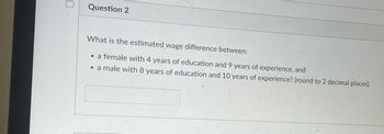
Transcribed Image Text:Question 2
What is the estimated wage difference between:
• a female with 4 years of education and 9 years of experience, and
• a male with 8 years of education and 10 years of experience? (round to 2 decimal places).
Expert Solution
This question has been solved!
Explore an expertly crafted, step-by-step solution for a thorough understanding of key concepts.
Step by stepSolved in 2 steps

Knowledge Booster
Similar questions
- Consider the population regression of log earnings [Y;, where Y,= In(Earnings,;)] against two binary variables: whether a worker is married (D₁, where D₁;= 1 if the th person is married) and the worker's gender (D2;, where D₂;= 1 if the th person is female), and the product of the two binary variables Y₁ = Po+B₁D₁+P₂D2i + P3 (D₁¡ × D₂i) + Hi- The interaction term: O A. indicates the effect of being married on log earnings. B. does not make sense since it could be zero for married males. C. allows the population effect on log earnings of being married to depend on gender. D. cannot be estimated without the presence of a continuous variable.arrow_forwardSuppose we are interested in evaluating the impact on wages of being a college graduate and of residing in California. To this end we define the following dummy variables if college graduate if not college graduate coll = ncoll = if not college graduate if college graduate 1 cali = if residing in California S 1 if not residing in California ncali = if not residing in California if residing in California and for wages denoting yearly wages, we estimate the following model of returns to education wages = B1 coll+ B2ncoll + B3 cali + B4(coll x cali) + e where E[e|coll, cali] = 0. Which parameter or combination of parameters measures the increase in expected wages from obtaining a college degree (comparing to not having a college degree) when residing California? O a. None of the other options is correct O b. Bi – B2 O c. B1 – B2 + ß4 O d. B4 O e. Bi + B3 – ßi – B4 O f. Bi + B4 – ß2 – B4 Clear my choicearrow_forwardThe question is the last bolded test. You need the previous questions to answer the last. Thank you for your time and help. You are the manager of a firm that sells CR2032 batteries for car key fobs and other electronic goods. You typically sell the fobs for $7 for a four-pack and sell an average of 27,192 four-packs per month. Due to increased labor costs, you decide to raise the price to $9 per four-pack. When you do this your monthly sales fall to 22,248 four-packs Assuming that your firm’s demand function is linear (i.e., takes the form ), calculate the linear demand function 22,248-27,192/9-7= -4944/2= -2472 Demand equation as 27,192 = a-2472(7) => a=27192+17304 =>a=44,496 27192= -2472x7+b 27192= -17304+b 27192+17304=44,496 Demand function is Q= -2472P+44,496 . Using the demand function that you estimated in the previous problem Calculate demand and total revenue when the price is $7 Q= -2472x7+44,496= -17,304+44,496= 27,192 Total revenue=PxQ=7x27,192=…arrow_forward
- Consider the following panel model to examine the effect of retirement on consumption expenditure, consit, of individual i over years t=1,…,3: (B1) log(consit) = β0 + β1retiredit + β2ageit + β3marriedit + β4healthit + δ1Yr2t + δ2Yr3t + ai + uit Where: retiredit is a dummy variable equal to 1 if individual i is retired on year t and 0 otherwise ageit is the individual's age in years marriedit is an indicator variable for whether the individual is married (1) or not (0) in year t healthit is an indicator variable equal to 1 if the individual is in 'good health' and 0 otherwise Yr2 is a dummy variable equal to 1 in year t=2 and 0 otherwise Yr3 is a dummy variable equal to 1 in year t=3 and 0 otherwise We obtain the following results when we estimate Model (B1) using RE and FE methods: Variable Random Effects Fixed Effects retired -0.072*** (0.024) -0.054** (0.025) age -0.008*** (0.003) - married 0.031*** (0.010) 0.028 (0.022) health 0.050*** (0.021) 0.052***…arrow_forwardYou are given a sample of 600 working individuals, with data on their location and earnings. You construct the following model: wage=Bo+Binorth+u, where the dependent variable is the annual earnings (wage) in $1,000. The explanatory variable is north (which equals one if a worker lives in the north, and equals zero otherwise). An OLS regression yields B 24.8. B₁ = 2.1. = As we have learned in class, education matters a lot in explaining wages-more years of education lead to higher wages. In the above econometric model, education belongs to the error term, u. We also know that in our population of interest, workers in the north have lower drop-out rates than workers in the south. These facts imply that B₁ is biased and inconsistent because the estimation is subject to omitted variable bias. The correct model should be: wage Bo+Binorth + B₂educ + e, where educ denotes the number of years of education. The OLS estimate of B1 from our incorrect model presented at the beginning of this…arrow_forward1. Suppose output (Q) is related to labor (L) and capital (K) in the following nonlinear way: Q = albKc When taking log to this equation, it is transformed into a linear LnQ = Ina + b In(L) + c Ln (K) One hundred twenty-three observations are used to obtain the following regression results: Dependant Variable: Observations: Variable Intercept L K Q 123 5.5215 Parameter Standard Estimate error 0.650 R-square 0.350 0.7547 0.9750 0.2950 0.1450 F-ratio 184.56 t-ratio 5.66 2.20 2.41 p-value on F 0.00001 p-value 0.0001 0.0295 0.0173 a. Write the regression equation based on the output either in the transformed linear form or the original non-linear form.arrow_forward
- Assume that the coefficient estimated in the second regression is correct. Forget about the effect of the Return variable, whose effect seems small and statistically insignificant. Calculate the correlation between Female and In(MarketValue) using the omitted variable bias equation. Let X Female, u=MarketValue, and =0.51. The correlation between Female and In(MarketValue), Px is -0.333. (Round your response to three decimal places.) Are large firms more likely to have female top executives than small firms? A. Yes. B. There is no relationship between the genders. C. No.arrow_forwardWhen labor usage is at 12units, the output is 36 units. From this, we may infer that. A) the marginal product of labor is 3 b) the total product of labor is 1/3 c)the average product of labor is 3 d) none of the abovearrow_forwardScenario 38-1. Consider the following OLS model applied to the data for workers wages and years of schooling, where e; stands for the residual: WAGE = -10.7+3.16 x SCHOOL + e. (20.7) (1.35) Refer to Scenario 38-1. Suppose that the residual term has a zero mean and is uncorrelated with the independent variable. According to the estimated model, each year of schooling decreases a worker's wage by $3.16. 000 decreases a worker's wage by $10.7. increases a worker's wage by $3.16. increases a worker's wage by $10.7.arrow_forward
arrow_back_ios
arrow_forward_ios
Recommended textbooks for you

 Principles of Economics (12th Edition)EconomicsISBN:9780134078779Author:Karl E. Case, Ray C. Fair, Sharon E. OsterPublisher:PEARSON
 Engineering Economy (17th Edition)EconomicsISBN:9780134870069Author:William G. Sullivan, Elin M. Wicks, C. Patrick KoellingPublisher:PEARSON
 Principles of Economics (MindTap Course List)EconomicsISBN:9781305585126Author:N. Gregory MankiwPublisher:Cengage Learning
 Managerial Economics: A Problem Solving ApproachEconomicsISBN:9781337106665Author:Luke M. Froeb, Brian T. McCann, Michael R. Ward, Mike ShorPublisher:Cengage Learning
 Managerial Economics & Business Strategy (Mcgraw-...EconomicsISBN:9781259290619Author:Michael Baye, Jeff PrincePublisher:McGraw-Hill Education


Principles of Economics (12th Edition)
Economics
ISBN:9780134078779
Author:Karl E. Case, Ray C. Fair, Sharon E. Oster
Publisher:PEARSON

Engineering Economy (17th Edition)
Economics
ISBN:9780134870069
Author:William G. Sullivan, Elin M. Wicks, C. Patrick Koelling
Publisher:PEARSON

Principles of Economics (MindTap Course List)
Economics
ISBN:9781305585126
Author:N. Gregory Mankiw
Publisher:Cengage Learning

Managerial Economics: A Problem Solving Approach
Economics
ISBN:9781337106665
Author:Luke M. Froeb, Brian T. McCann, Michael R. Ward, Mike Shor
Publisher:Cengage Learning

Managerial Economics & Business Strategy (Mcgraw-...
Economics
ISBN:9781259290619
Author:Michael Baye, Jeff Prince
Publisher:McGraw-Hill Education