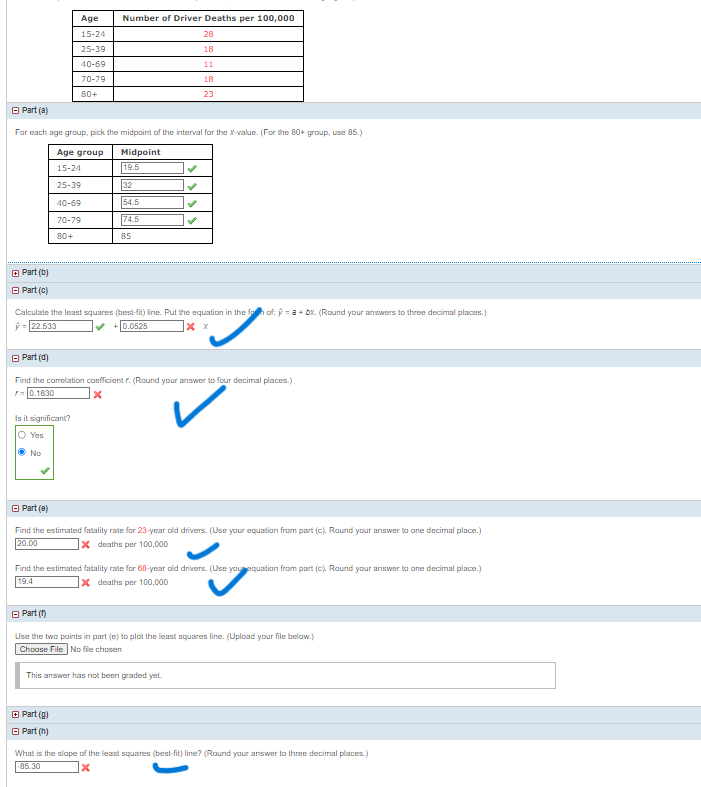
Part (a) Part (b) Part (c) For each age group, pick the midpoint of the interval for the X-value. (For the 80+ group, use 85.) Midpoint 19.5 32 54.5 74.5 Age 15-24 25-39 40-69 70-79 80+ Yes Age group 15-24 25-39 Is it significant? No 40-69 70-79 80+ Number of Driver Deaths per 100,000 Calculate the least squares (best-fit) line. Put the equation in the fhof: 9-abx. (Round your answers to three decimal places.) -22.533 0.0525 x x Part (d) Find the correlation coefficient r. (Round your answer to four decimal places.) -0.1830 x 85 28 18 11 18 23 Part (g) Part (0) Find the estimated fatality rate for 23-year old drivers. (Use your equation from part (c). Round your answer to one decimal place.) x deaths per 100,000 20.00 Find the estimated fatality rate for 68-year old drivers. (Use you equation from part (e), Round your answer to one decimal place.) 19.4 * deaths per 100,000 Part (1) Use the two points in part (e) to plot the least squares line. (Upload your file below.) Choose File No fie chosen This answer has not been graded yet.

Apex Learning - Courses course.apexlearning.com/public/activity/2002003/assessment L 2.2.3 Quiz: Graphing Functions -5 5. -5 Which statement best describes the function? O A. The function is never negative. O B. The function is negative when x > 0. O C. The function is negative when x 0. O D. The function is negative when x< 0. E PREVIOUS

Evan is investigating how long his phone's battery lasts (in hours) for various brightness levels (on a scale of 0-100). His data is displayed in the table and graph below. Brightness Level (x) 17 26 30 35 36 37 45 94 Hours (y) 6.7 5.9 5.8 4.5 6.8 6.1 3.8 2.1   10203040506070809010011012345678910-1Brightness LevelHours a) Find the equation for the line of best fit. Keep at least 4 decimals for each parameter in the equation.    b) Interpret the slope in context. Evan should expect -0.0604 hours per brightness level. Evan should expect -0.0604 brightness level per hour.   c) What does the equation predict for the number of hours the phone will last at a brightness level of 36?  hours