
MATLAB: An Introduction with Applications
6th Edition
ISBN: 9781119256830
Author: Amos Gilat
Publisher: John Wiley & Sons Inc
expand_more
expand_more
format_list_bulleted
Related questions
Concept explainers
Question
In the packaging department of a large aircraft parts distributor, a fairly reliable estimate of packaging and processing costs can be determined by knowing the weight of an order. Thus, the weight is a cost driver that accounts for a sizable fraction of the packaging and processing costs at this company. Data for the past 10 orders are given as follows. Solve, a. Estimate the b0 and b1 coefficients, and determine the linear regression equation to fit these data. b. What is the
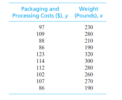

Transcribed Image Text:Packaging and
Processing Costs ($), y (Pounds), x
Weight
97
230
109
280
88
210
86
190
123
320
114
300
112
280
102
260
107
270
86
190
Expert Solution
This question has been solved!
Explore an expertly crafted, step-by-step solution for a thorough understanding of key concepts.

This is a popular solution

Trending nowThis is a popular solution!

Step by stepSolved in 3 steps with 5 images

Knowledge Booster


Learn more about
Need a deep-dive on the concept behind this application? Look no further. Learn more about this topic, statistics and related others by exploring similar questions and additional content below.Similar questions
- The datasetBody.xlsgives the percent of weight made up of body fat for 100 men as well as other variables such as Age, Weight (lb), Height (in), and circumference (cm) measurements for the Neck, Chest, Abdomen, Ankle, Biceps, and Wrist. We are interested in predicting body fat based on abdomen circumference. Find the equation of the regression line relating to body fat and abdomen circumference. Make a scatter-plot with a regression line. What body fat percent does the line predict for a person with an abdomen circumference of 110 cm? One of the men in the study had an abdomen circumference of 92.4 cm and a body fat of 22.5 percent. Find the residual that corresponds to this observation. Bodyfat Abdomen 32.3 115.6 22.5 92.4 22 86 12.3 85.2 20.5 95.6 22.6 100 28.7 103.1 21.3 89.6 29.9 110.3 21.3 100.5 29.9 100.5 20.4 98.9 16.9 90.3 14.7 83.3 10.8 73.7 26.7 94.9 11.3 86.7 18.1 87.5 8.8 82.8 11.8 83.3 11 83.6 14.9 87 31.9 108.5 17.3…arrow_forwardPersonal wealth tends to increase with age as older individuals have had more opportunities to earn and invest than younger individuals. The following data were obtained from a random sample of eight individuals and records their total wealth (Y) and their current age (X). Data provided in the image. a. State the estimated regression line and interpret the slope coefficient.b. What is the estimated total personal wealth when a person is 50 years old?c. What is the value of the coefficient of determination? Interpret it. d. Test whether there is a significant relationship between wealth and age at the 10%significance level. Perform the test using the following six steps. Step 1. Statement of the hypothesesStep 2. Standardised test statisticStep 3. Level of significanceStep 4. Decision. Step 5. Calculation of test statistic. Step 6. Conclusion Please solve the d) part only.arrow_forwardPlease provide solution and logic for questions attached, thanks!arrow_forward
- The value of a sports franchise is directly related to the amount of revenue that a franchise can generate. The following data represents the value in 2014 (in $millions) and the annual revenue (in $millions) for the 30 Major League Baseball franchises. Suppose you want to develop a simple linear regression model to predict franchise value based on annual revenue generated. Team Revenue Value Baltimore 245 1000 Boston 370 2100 Chicago White Sox 227 975 Cleveland 207 825 Detroit 254 1125 Houston 175 800 Kansas City 231 700 Los Angeles Angels 304 1300 Minnesota 223 895 New York Yankees 508 3200 Oakland 202 725 Seattle 250 1100 Tampa Bay 188 625 Texas 266 1220 Toronto 226 870 Arizona 211 840 Atlanta 267 1150 Chicago Cubs 302 1800 Cincinnati 227 885 Colorado…arrow_forwardConsider the following sample of production volumes and total cost data for a manufacturing operation. Production Volume Total Cost (units) ($) 400 4,100 450 5,000 550 5,400 600 5,900 700 6,500 750 6,900 This data was used to develop an estimated regression equation, ŷ = 1,401.33 + 7.36x, relating production volume and cost for a particular manufacturing operation. Use a = 0.05 to test whether the production volume is significantly related to the total cost. (Use the F test.) State the null and alternative hypotheses. Hoi Bo = 0 Ha: Bo + 0 O Ho: B1 + 0 H: B1 = 0 Ho: B1 20 H: B, < 0 1 Ho: Bo + 0 Hạ: Bo = 0 Hoi B1 = 0 Set up the ANOVA table. (Round your p-value to three decimal places and all other values to two decimal places.) Source Sum Degrees of Freedom Mean F p-value of Variation of Squares Square Regressionarrow_forwardA sales manager collected the following data on x = years of experience and y = annual sales ($1,000s). The estimated regression equation for these data is ý = 81 + 4x. Years of Annual Sales Salesperson Experience ($1,000s) 80 3 97 3 102 4 4 102 103 6. 8 101 10 119 8 10 123 9. 11 127 10 13 136 (a) Compute SST, SSR, and SSE. SST = SSR = SSE = (b) Compute the coefficient of determination r2. (Round your answer to three decimal places.) r2 = Comment on the goodness of fit. (For purposes of this exercise, consider a proportion large if it is at least 0.55.) O The least squares line did not provide a good fit as a small proportion of the variability in y has been explained by the least squares line. The least squares line provided a good fit as a large proportion of the variability in y has been explained by the least squares line. The least squares line provided a good fit as a small proportion of the variability in y has been explained by the least squares line. The least squares line did…arrow_forward
arrow_back_ios
arrow_forward_ios
Recommended textbooks for you
- MATLAB: An Introduction with ApplicationsStatisticsISBN:9781119256830Author:Amos GilatPublisher:John Wiley & Sons Inc
 Probability and Statistics for Engineering and th...StatisticsISBN:9781305251809Author:Jay L. DevorePublisher:Cengage Learning
 Statistics for The Behavioral Sciences (MindTap C...StatisticsISBN:9781305504912Author:Frederick J Gravetter, Larry B. WallnauPublisher:Cengage Learning
  Elementary Statistics: Picturing the World (7th E...StatisticsISBN:9780134683416Author:Ron Larson, Betsy FarberPublisher:PEARSON
 The Basic Practice of StatisticsStatisticsISBN:9781319042578Author:David S. Moore, William I. Notz, Michael A. FlignerPublisher:W. H. Freeman
 Introduction to the Practice of StatisticsStatisticsISBN:9781319013387Author:David S. Moore, George P. McCabe, Bruce A. CraigPublisher:W. H. Freeman
MATLAB: An Introduction with Applications
Statistics
ISBN:9781119256830
Author:Amos Gilat
Publisher:John Wiley & Sons Inc
Probability and Statistics for Engineering and th...
Statistics
ISBN:9781305251809
Author:Jay L. Devore
Publisher:Cengage Learning
Statistics for The Behavioral Sciences (MindTap C...
Statistics
ISBN:9781305504912
Author:Frederick J Gravetter, Larry B. Wallnau
Publisher:Cengage Learning
Elementary Statistics: Picturing the World (7th E...
Statistics
ISBN:9780134683416
Author:Ron Larson, Betsy Farber
Publisher:PEARSON
The Basic Practice of Statistics
Statistics
ISBN:9781319042578
Author:David S. Moore, William I. Notz, Michael A. Fligner
Publisher:W. H. Freeman
Introduction to the Practice of Statistics
Statistics
ISBN:9781319013387
Author:David S. Moore, George P. McCabe, Bruce A. Craig
Publisher:W. H. Freeman