MATLAB: An Introduction with Applications
6th Edition
ISBN: 9781119256830
Author: Amos Gilat
Publisher: John Wiley & Sons Inc
expand_more
expand_more
format_list_bulleted
Question
please answer these questions step by step please with full calculations as soon as possible

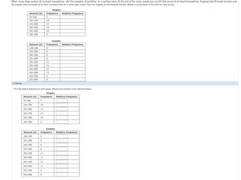
Transcribed Image Text:Often, cruise ships conduct all on-board transactions, with the exception of gambling, on a cashless basis. At the end of the cruise, guests pay one bill that covers all on-board transactions. Suppose that 58 single travelers and
80 couples were surveyed as to their on-board bills for a seven-day cruise from Los Angeles to the Mexican Riviera. Below is a summary of the bills for each group.
Singles
Amount ($)
51-100
Frequency
Relative Frequency
5
101-150
10
151-200
14
201-250
14
251-300
10
301-350
5
Couples
Amount ($)
Frequency
Relative Frequency
100-150
6
151-200
6
201-250
6
251-300
6
301-350
11
351-400
11
401-450
11
451-500
11
501-550
6
551-600
6
Part (a)
Fill in the relative frequency for each group. (Round your answers to four decimal places.)
Singles
Amount ($)
Frequency
Relative Frequency
51-100
5
101-150
10
151-200
14
201-250
14
251-300
10
301-350
5
Couples
Amount ($)
Frequency
Relative Frequency
100-150
6
151-200
6
201-250
6
251-300
6
301-350
11
351-400
11
401-450
11
451-500
11
501-550
6
551-600

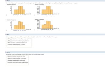
Transcribed Image Text:Part (e)
Construct a new graph for the couples by hand. Since each couple is paying for two individuals, instead of scaling the x-axis by $50, scale it by $100. Use relative frequency on the y-axis.
Relative Frequency
Relative Frequency
20
15
0.25
0.20
0.15
10
0.10
5
0.05
0
Amount ($)
0.00
Amount ($)
100 200 300 400 500 600
100 200 300 400 500 600
Relative Frequency
Relative Frequency
0.30
0.25
20
0.20
15
0.15
10
0.10
5
0.05
0.00
Amount ($)
0
Amount ($)
100 200 300 400 500 600
100 200 300 400 500 600
Part (f)
Compare the graph for the singles with the new graph for the couples. List two similarities between the graphs. (Select all that apply.)
Both graphs show lowest relative frequencies near the tails.
Both graphs represent a relative frequency distribution.
Both graphs show a wide spread of data values.
☐ The center value of each graph is the same.
Part (g)
By scaling the couples graph differently, how did it change the way you compared it to the singles?
O It changed the center of the Couples graph.
O It changed the skewness of the Couples graph.
O It changed the spread of the Couples graph.
O It changed the number of intervals being compared.
Expert Solution
This question has been solved!
Explore an expertly crafted, step-by-step solution for a thorough understanding of key concepts.
Step by stepSolved in 2 steps

Knowledge Booster
Similar questions
- Your neighborhood has seen some growth in squirrel population over the past couple years. Two years ago you noticed eight squirrels living in your and your neighbor’s yards. Last year you counted 12 squirrels. Currently, there are 18 squirrels that live in the yards. Write an equation representing this situation. If this rate of growth continues, how many squirrels should you expect to see 5 years from now?arrow_forwardYour grandmother invests part of $4,063 at 8.0% and the rest at 6.5%. Her annual interest income from both accounts is $299. How much money did she invest at 8.0\% ?arrow_forwardPlease include all stepsarrow_forward
- The rental agency will earn a maximum income of $ when it charges s per day.arrow_forwardplease don't make calculations long make it short and simple Please please answer fast please answer as fast as possible please it's super important and super urgent Please please answer as fast as possible please I’m begging please answer fast I need it in less than 40 minutesarrow_forwardA person invested $7,400 in an account growing at a rate allowing the money to double every 6 years. How much money would be in the account after 4 years, to the nearest dollar?arrow_forward
arrow_back_ios
arrow_forward_ios
Recommended textbooks for you
 MATLAB: An Introduction with ApplicationsStatisticsISBN:9781119256830Author:Amos GilatPublisher:John Wiley & Sons Inc
 Probability and Statistics for Engineering and th...StatisticsISBN:9781305251809Author:Jay L. DevorePublisher:Cengage Learning
 Statistics for The Behavioral Sciences (MindTap C...StatisticsISBN:9781305504912Author:Frederick J Gravetter, Larry B. WallnauPublisher:Cengage Learning
 Elementary Statistics: Picturing the World (7th E...StatisticsISBN:9780134683416Author:Ron Larson, Betsy FarberPublisher:PEARSON
 The Basic Practice of StatisticsStatisticsISBN:9781319042578Author:David S. Moore, William I. Notz, Michael A. FlignerPublisher:W. H. Freeman
 Introduction to the Practice of StatisticsStatisticsISBN:9781319013387Author:David S. Moore, George P. McCabe, Bruce A. CraigPublisher:W. H. Freeman

MATLAB: An Introduction with Applications
Statistics
ISBN:9781119256830
Author:Amos Gilat
Publisher:John Wiley & Sons Inc

Probability and Statistics for Engineering and th...
Statistics
ISBN:9781305251809
Author:Jay L. Devore
Publisher:Cengage Learning

Statistics for The Behavioral Sciences (MindTap C...
Statistics
ISBN:9781305504912
Author:Frederick J Gravetter, Larry B. Wallnau
Publisher:Cengage Learning

Elementary Statistics: Picturing the World (7th E...
Statistics
ISBN:9780134683416
Author:Ron Larson, Betsy Farber
Publisher:PEARSON

The Basic Practice of Statistics
Statistics
ISBN:9781319042578
Author:David S. Moore, William I. Notz, Michael A. Fligner
Publisher:W. H. Freeman

Introduction to the Practice of Statistics
Statistics
ISBN:9781319013387
Author:David S. Moore, George P. McCabe, Bruce A. Craig
Publisher:W. H. Freeman