
MATLAB: An Introduction with Applications
6th Edition
ISBN: 9781119256830
Author: Amos Gilat
Publisher: John Wiley & Sons Inc
expand_more
expand_more
format_list_bulleted
Related questions
Question
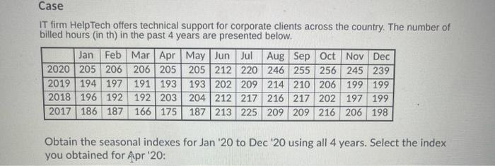

Transcribed Image Text:Case
IT firm HelpTech offers technical support for corporate clients across the country. The number of
billed hours (in th) in the past 4 years are presented below.
246 255 256 245 239
Jan Feb Mar Apr May Jun Jul Aug Sep Oct Nov Dec
2020 205 206 206 205 205 212 220
2019 194 197 191 193
2018 196 192 192 203
2017 186 187 166 175
193 202 209 214 210 206 199 199
204 212 217 216 217 202 197 199
187 213 225 209 209 216 206 198
Obtain the seasonal indexes for Jan '20 to Dec '20 using all 4 years. Select the index
you obtained for Apr '20:

Transcribed Image Text:Obtain the optimal parameters (alpha and beta) using Excel's Solver that would
minimize the previously calculated 2020 MSE.
alpha = 1, beta = 0
alpha=0.342, beta = 0.631
alpha=0, beta 1
alpha 0.908, beta = 0.337
=
Expert Solution
This question has been solved!
Explore an expertly crafted, step-by-step solution for a thorough understanding of key concepts.

Step by stepSolved in 3 steps with 2 images

Knowledge Booster

Similar questions
- (3) The approximate enrollment, in millions between the years 2009 and 2018 is provided by a linear model Y3D0.2309x+18.35 Where x-0 corresponds to 2009, x=1 to 2010, and so on, and y is in millions of students. Use the model determine projected enrollment for the year 2014. 近arrow_forwardCarbon-14 has a half-life of 5730 years, with k=-0.000120968. 1 of the initial amount of carbon-14 that it contained when the A fossil human jawbone contains 1000 person was alive. Determine the approximate age of the fossil? Select one: а. 42 305 yеars b. None of these с. 12 004 years d. 57 103 years е. 13 511 yearsarrow_forwardIn a certain region, about 6% of a city's population moves to the surrounding suburbs each year, and about 2% of the suburban population moves into the city. In 2020, there were 9,750,000 residents in the city and 900,000 residents in the suburbs. Set up a difference equation that describes this situation, where x is the initial population in 2020. Then estimate the populations in the city and in the suburbs two years later, in 2022. (Ignore other factors that might influence the population sizes.) Set up a difference equation that describes this situation, where x is the initial population in 2020. x₁ = Mx0 = (Type an integer or decimal for each matrix element. Do not perform the calculation.)arrow_forward
- From 2000 through 2009, the population of State A grew more slowly than that of State B. Models that represent the populations of the two states are given by P = 37.5t + 6075 State A P = 168.2t + 5138 State B where P is the population (in thousands) and t represents the year, with t = 0 corresponding to 2000. Use the models to estimate when the population of State B first exceeded the population of State A. (Round your answer to the nearest year.)arrow_forwardThe same disease is spreading through two populations, say Pi and P2, with the same size. You may assume that the spread of the disease is well described by the SIR model. dSa - BaSaIa dt dla - dt dRa YaIa dt with Sa(0) + I.(0) + R.(0) = N where N denotes the fixed population size. The subscript a identifies the population P or P2. For example, if a = 1, the variables are related to P1. Assume that S1 (0) = S2 (0) and I1(0) = I½(0) and that no interventions such as quarantine or vaccination have been implemented. If the difference in the spread of the disease is due only to the poor over-all health of a population, which population has the best over-all health of the two populations? - Susceptible Population 1 - Susceptible Population 2 700 600 500 400 300 200 100 10 15 20 t P1. P2. Susceptiblearrow_forwardPlease calculate the following Chi Square equations. 1. Chi Square Single Sample Physical activity generally declines when students leave high school and enroll in college. This suggests that college is an ideal setting to promote physical activity. One study examined the level of physical activity in a sample of 570 college students. Use the hypothesis steps provided in the video to determine whether there is a significant difference in physical activity among college students. State whether you reject or fail to reject the null hypothesis.arrow_forward
- Use the following linear regression equation to answer the questions. x1 = 2.0 + 3.6x2 – 7.8x3 + 2.1x4 a) Suppose x3 and x4 were held at fixed but arbitrary values and x2 increased by 1 unit. What would be the corresponding change in x1?b) Suppose x2 increased by 2 units. What would be the expected change in x1?c) Suppose x2 decreased by 4 units. What would be the expected change in x1?arrow_forwardGiven a 98% level of confidence, find the critical value Zα/2 and also solve when given a 93% level of confidence, find the critical value Zα/2.arrow_forwardIf L(x)=mx+b is the linearization of the cube root of 3x+1 at x=333 , then b=arrow_forward
arrow_back_ios
arrow_forward_ios
Recommended textbooks for you
- MATLAB: An Introduction with ApplicationsStatisticsISBN:9781119256830Author:Amos GilatPublisher:John Wiley & Sons Inc
 Probability and Statistics for Engineering and th...StatisticsISBN:9781305251809Author:Jay L. DevorePublisher:Cengage Learning
 Statistics for The Behavioral Sciences (MindTap C...StatisticsISBN:9781305504912Author:Frederick J Gravetter, Larry B. WallnauPublisher:Cengage Learning
  Elementary Statistics: Picturing the World (7th E...StatisticsISBN:9780134683416Author:Ron Larson, Betsy FarberPublisher:PEARSON
 The Basic Practice of StatisticsStatisticsISBN:9781319042578Author:David S. Moore, William I. Notz, Michael A. FlignerPublisher:W. H. Freeman
 Introduction to the Practice of StatisticsStatisticsISBN:9781319013387Author:David S. Moore, George P. McCabe, Bruce A. CraigPublisher:W. H. Freeman
MATLAB: An Introduction with Applications
Statistics
ISBN:9781119256830
Author:Amos Gilat
Publisher:John Wiley & Sons Inc
Probability and Statistics for Engineering and th...
Statistics
ISBN:9781305251809
Author:Jay L. Devore
Publisher:Cengage Learning
Statistics for The Behavioral Sciences (MindTap C...
Statistics
ISBN:9781305504912
Author:Frederick J Gravetter, Larry B. Wallnau
Publisher:Cengage Learning
Elementary Statistics: Picturing the World (7th E...
Statistics
ISBN:9780134683416
Author:Ron Larson, Betsy Farber
Publisher:PEARSON
The Basic Practice of Statistics
Statistics
ISBN:9781319042578
Author:David S. Moore, William I. Notz, Michael A. Fligner
Publisher:W. H. Freeman
Introduction to the Practice of Statistics
Statistics
ISBN:9781319013387
Author:David S. Moore, George P. McCabe, Bruce A. Craig
Publisher:W. H. Freeman