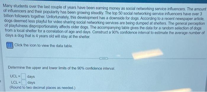
Many students over the last couple of years have been earning money as social networking service influencers. The amou of influencers and their popularity has been growing steadily. The top 50 social networking service influencers have over 3 billion followers together. Unfortunately, this development has a downside for dogs. According to a recent newspaper articl dogs deemed less playful for video sharing social networking services are being dumped at shelters. The general perceptic of playfulness disproportionately affects older dogs. The accompanying table gives the data for a random selection of dogs from a local shelter for a correlation of age and days. Construct a 90% confidence interval to estimate the average number days a dog that is 4 years old will stay at the shelter. Click the icon to view the data table. Determine (XXX) the upper and lower limits of the 90% confidence interval. UCL = days

The U.S. Department of Transportation, National Highway Traffic Safety Administration, reported that 77% of all fatally injured automobile drivers were intoxicated. A random sample of 26 records of automobile driver fatalities in Kit Carson County, Colorado, showed that 14 involved an intoxicated driver. Do these data indicate that the population proportion of driver fatalities related to alcohol is less than 77% in Kit Carson County? Use ? = 0.01. Solve the problem using both the traditional method and the P-value method. Since the sampling distribution of p̂ is the normal distribution, you can use critical values from the standard normal distribution as shown in the table of critical values of the z distribution. (Round the test statistic and the critical value to two decimal places. Round the P-value to four decimal places.)   test statistic =   critical value =   P-value =

Which are the ultimate tools that are being brought in business analytics?

What is business analytics? Briefly describe the domain of the major fields of business analytics databases and data warehousing, descriptive, predictive, and prescriptive analytics.

Suppose Laura, a facilities manager at a health and wellness company, wants to estimate the difference in the average amount of time that men and women spend at the company's fitness centers each week. Laura randomly selects 15 adult male fitness center members from the membership database and then selects 15 adult female members from the database. Laura gathers data from the past month containing logged time at the fitness center for these members. She plans to use the data to estimate the difference in the time men and women spend per week at the fitness center. The sample statistics are summarized in the table. Population Populationdescription Population mean(unknown) Samplesize Sample mean(min) Sample standarddeviation (min) 11 male μ1 n=15 x¯1=137.7 s=51.7 22 female μ2 n=15 x¯2=114.6 s=34.2   df=24.283   The population standard deviations are unknown and unlikely to be equal, based on the sample data. Laura plans to use the two-sample ?-t-procedures to estimate the…

R Studio       library(poliscidata)       2. (Dataset: nes. Variables: dhsinvolv_message, polknow_combined.) Online political activism is a relatively new phenomenon. In recent years, online social networks like Facebook and Twitter have become part of our everyday experiences and, for many people, a forum for political news and debate. From your own personal experiences, you may have some impressions about who is likely to post political messages online, but our personal perspectives are bound to be limited and incomplete. Let's use the nes dataset to gain a better understanding of who uses social media to promote political ideas. Survey participants were asked whether they had posted a political message on Facebook or Twitter in the last 4 years and the dhsinvolv_message variable recorded their responses.        1. According to the nes dataset, roughly 20% of respondents indicated that they had posted a social media message about politics in the past 4 years. If the probability of an…

Approval 2008. Of all the post–World War II presidents,Richard Nixon had the highest disapproval rating near theend of his presidency. His disapproval rating peaked at 66% in July 1974, just before he resigned. This percent-age has been considered by some pundits as a high water mark for presidential disapproval. However, in April 2008,George W. Bush’s disapproval rating peaked at 69%,according to a Gallup poll of 1016 voters. Pundits starteddiscussing whether his rating was discernibly worse thanthe previous high water mark of 66%. What do you think?

The website Data USA stated that in 2016, Texas had the lowest number of adults with a serious mental illness with an average of M=3.26% of the population affected. The state of Texas wants to test if they have a significantly decreased number of mental illness patients compared with the states with the (n=8) highest level of mental illness found. In 2016 the following states had the highest level of adult patients with mental illness: Arkansas= 5.45%, Montana=5.34%, Vermont=5.32%, Oregon=5.19%, Utah=5.2%, Ohio=5.13, Kentucky=5.25% West Virginia=5.18%. The alpha level for the study was set to α=.05 for the criteria. a. State the hypotheses of the study. b. Find the critical t value for this study c. Compute the one-sample t test. (Again calculate sample SD or s - and get SEM before calculating t.) d. Compute the Cohen's d for the data (even if not significant) e. State the results - is the sample significantly higher? Do you reject the null hypothesis? Report the t test results in APA…

Suppose you are conducting a study about how the average US worker spends time over the course of a workday. You are interested in how much time workers spend per day on personal calls, emails, and social networking websites, as well as how much time they spend socializing with coworkers versus actually working. The most recent census provides data for the entire population of US workers on variables such as travel time to work, time spent at work, and break time at work. The census, however, does not include data on the variables you are interested in, so you obtain a random sample of 102 full-time workers in the United States and ask about personal calls, emails, and so forth. You are curious about how your sample compares with the census, so you also ask the workers the same questions about work that are asked in the census. Suppose the mean travel time to work from the most recent census is 24.1 minutes, with a standard deviation of 4.5 minutes. Your sample of 102 US workers…

Several epidemiologists conducted a cohort study of the effect of mercury exposure on the development of brain cancer. Subjects were followed for ten years. There were a total of 150,000 people in the study. Among the subjects, 76,000 were exposed to mercury and the rest were not. 52,000 of those exposed to mercury developed brain cancer, and only 1,200 of those unexposed to mercury developed brain cancer.  Please create a two-by-two table. Calculate the relative risk and interpret it in a sentence. Calculate the attributable risk and interpret. Calculate the percent attributable risk and interpret. Assume that 30% of people in Rhode Island are exposed to mercury, calculate and interpret the population attributable risk and calculate and interpret the percent population attributable risk.