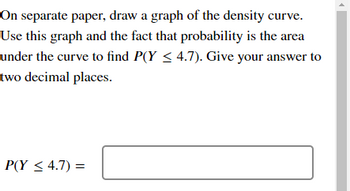
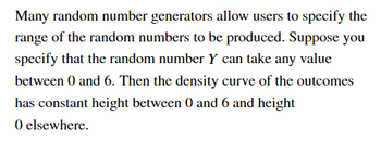
On separate paper, draw a graph of the density curve.Use this graph and the fact that probability is the areaunder the curve to find P(Y ≤ 4.7). Give your answer totwo decimal places.P(Y ≤ 4.7) = Many random number generators allow users to specify therange of the random numbers to be produced. Suppose youspecify that the random number Y can take any valuebetween 0 and 6. Then the density curve of the outcomeshas constant height between 0 and 6 and heightO elsewhere.

The random number Y can take any value between 0 and 6.The density curve has a constant height…

Answered: Many random number generators allow…

MATLAB: An Introduction with Applications

6th Edition

ISBN:9781119256830

Author:Amos Gilat

Publisher:Amos Gilat

Chapter1: Starting With Matlab

Section: Chapter Questions

Problem 1P

See similar textbooks

Similar questions

You study a population and are interested in the proportionpthat has a certain characteristic. You are unaware that this proportion of the population isp=0.67. You have taken a random sample of sizen & 129of the population and determined that the proportion of the sample having the characteristic isp=0.73. His sample is Sample 1 in the following table. (In the table, Sample 1 is indicated by "M1", Sample 2 by "M2", and so on). (to) Based on Sample 1, plot the confidence intervals of80%and of95%for the population proportion. Use1,282for the critical value for the confidence interval of80%, and use1960 for the critical value for the confidence interval of95%. (If necessary, you can refer to a list of formulas.) • Write the upper limit and the lower limit on the graphs to indicate each confidence interval. Write the answers with two decimal places. • For the points ( ♦and ◆), write the population proportion,0.67. 0.47 0.47 80% confidence interval 0.65 X 0.84 0.84 0.47 0.47 95% confidence…
Let n be a random sample from the exp(0) Show that X is a sufficient statistic for
A deck has "b" black cards and "y" yellow cards. Given that cards are drawn at a random fashion without replacement. Find the average where after drawing a black card it is immediately followed by a yellow card
How many possible random samples of size n = 3 can be drawn from a population of size 10?
. Find the moment generating function about origin of the Poisson distribution.
Hi Please assi
Only parts D and E please.
Is the following random variable discrete or continuous? Let X represent the number of books in a random professor's office.
Let X₁, X₂.....X₁ be a random sample from an exponential distribution with parameter 8. Find the MLE for P(X≥1).
1. Provide the graphs for PDF and CDF of the random variable B which takes on values of 1 and 0 with probability of 0.40 and 0.60. (Don't forget the horizontal axis must be sorted).
A school district has a standardized test that it uses to determine placement into special classes. The superintendent is looking to determine whether male and female students have different scores on the test. The scores for a random sample of 25 male students and 25 female students are recorded. Assume that the scores are normally distributed for both male and female students. Let the male students be the first sample, and let the female students be the second sample. Is there enough evidence, at a = 0.01 to show a difference between male and female scores? Identify the degree of freedom and the critical value(s) to be used for this hypothesis test. Do not round; use the exact value from the t-table. Degree of freedom = Provide your answer below: Critical Value(s) = Males Females x1 = 168x2 = 171 $1 = 14 $2 = 17 n1 = 25 n2 = 25 Probability Degrees of Freedom 23 24 25 26 27 28 29 0.10 0.05 0.025 0.01 0.005 1.319 1.714 2.069 2.500 2.807 1.318 1.711 2.064 2.492 2.797 1.316 1.708 2.060…

Recommended textbooks for you

MATLAB: An Introduction with Applications

Statistics

ISBN:

9781119256830

Author:

Amos Gilat

Publisher:

John Wiley & Sons Inc

Probability and Statistics for Engineering and th…

Statistics

ISBN:

9781305251809

Author:

Jay L. Devore

Publisher:

Cengage Learning

Statistics for The Behavioral Sciences (MindTap C…

Statistics

ISBN:

9781305504912

Author:

Frederick J Gravetter, Larry B. Wallnau

Publisher:

Cengage Learning

MATLAB: An Introduction with Applications

Statistics

ISBN:

9781119256830

Author:

Amos Gilat

Publisher:

John Wiley & Sons Inc

Probability and Statistics for Engineering and th…

Statistics

ISBN:

9781305251809

Author:

Jay L. Devore

Publisher:

Cengage Learning

Statistics for The Behavioral Sciences (MindTap C…

Statistics

ISBN:

9781305504912

Author:

Frederick J Gravetter, Larry B. Wallnau

Publisher:

Cengage Learning

Elementary Statistics: Picturing the World (7th E…

Statistics

ISBN:

9780134683416

Author:

Ron Larson, Betsy Farber

Publisher:

PEARSON

The Basic Practice of Statistics

Statistics

ISBN:

9781319042578

Author:

David S. Moore, William I. Notz, Michael A. Fligner

Publisher:

W. H. Freeman

Introduction to the Practice of Statistics

Statistics

ISBN:

9781319013387

Author:

David S. Moore, George P. McCabe, Bruce A. Craig

Publisher:

W. H. Freeman

SEE MORE TEXTBOOKS

Many random number generators allow users to specify the range of the random numbers to be produced. Suppose you specify that the random number Y can take any value between 0 and 6. Then the density curve of the outcomes has constant height between 0 and 6 and height 0 elsewhere.