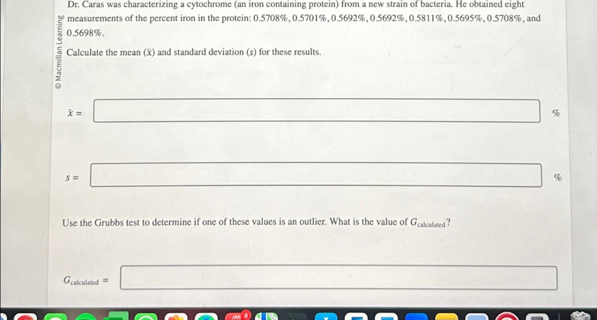
Macmillan LearningDr. Caras was characterizing a cytochrome (an iron containing protein) from a new strain of bacteria. He obtained eightmeasurements of the percent iron in the protein: 0.5708%, 0.5701%, 0.5692%, 0.5692%, 0.5811%, 0.5695%, 0.5708%, and0.5698%.Calculate the mean (x) and standard deviation (s) for these results.x =S=Use the Grubbs test to determine if one of these values is an outlier. What is the value of Gcalculated?Gcalculated =%%

Given that :The % of the iron in the protein for the eight measurements is given as: 0.5708%,…

Answered: Macmillan Learning Dr. Caras was…

MATLAB: An Introduction with Applications

6th Edition

ISBN:9781119256830

Author:Amos Gilat

Publisher:Amos Gilat

Chapter1: Starting With Matlab

Section: Chapter Questions

Problem 1P

See similar textbooks

Similar questions

To find the slope for predicting Y, we need to use the formula: slope = R* (sd2y / sd2x) where R is the correlation coefficient between X and Y, sd2x is the standard deviation of X squared, and sd2y is the standard deviation of Y squared. Given the values provided, we have: sd2x = 10.23 sd2y = 13.34 R2 = 0.14
Match the coefficient of determination to the scatter diagram. The scales on the x-axis and y-axis are the same for each scatter diagram. (a) R? = 0.12, (b) R² = 0.98, (c) R² = 1 %3D (a) Scatter diagram Explanatory (b) Scatter diagram II (c) Scatter diagram Explanatory II II Explanatory II aSuods asuodsəy Response
Thomas wants to compare the mean concentration of carbon monoxide (CO) on residential versus commercial streets, since these differ in terms of car traffic. In each of three neighborhoods of Montréal (named A, B, and C below), he randomly chooses four locations for each type of street, for a total of 24 observations (2 street types x 3 neighborhoods x 4 locations). At each location, he measures CO concentration in the air over a period of 10 hours (8:00 AM-6:00 PM), and obtains the following data (in ppm/h). Question: Test whether or not the difference between residential and commercial streets in mean atmospheric CO concentration is the same among the three neighborhoods, and whether or not CO concentration in the air is the same, on average, for the two types of streets. Note that Neighborhood is considered a random block factor in the ANOVA. Use significant level= 0.05.
Complete the FD table below and then: find 60th percentile: n = 30 = 15 (L=45 8-10-11-13. 1416. 4 6 Classes Frequency 2-4 5 Vies 5-7 you 2.11 5 classnumbers b U 16-2= class= W 14 FDT=2.8~3
Trace metals in drinking water affect the flavor and an unusually high concentration can pose a health hazard. Ten pairs of data were taken measuring zinc concentration in bottom water and surface water. Bottom 0.430 0.266 0.567 0.531 0.707 0.716 0.651 0.589 0.469 0.723 Surface 0.415 0.238 0.390 0.410 0.605 0.609 0.632 0.523 0.411 0.612 With the help of Mathematics and R Studio: Does the data suggest that the true average concentration in the bottom water is different than that of surface water? You can assume that the conditions for inference are met.
If X = 85, Y = 54, and Y' = 62, what is the residual score? a. -8 b. 23 c. 8 d. 31
In the General Social Survey, respondents were asked whether they favor cuts in governmental spending. Here is the output summarizing this variable: Statistics CUTS IN GOVT SPENDING. Valid 1375 Missing 1492 Mean 2.24 Median 2.00 Mode Percentiles 25 1.00 50 2.00 75 3.00 CUTS IN GOVT SPENDING. Cumulative Frequency Percent Valid Percent Percent Valid STRONGLY IN FAVOR 413 14.4 30.0 30.0 IN FAVOR 471 16.4 34.3 64.3 NEITHER 294 10.3 21.4 85.7 AGAINST 143 5.0 10.4 96.1 STRONGLY AGAINST 54 1.9 3.9 100.0 Total 1375 48.0 100.0 Missing JAP 1477 51.5 DK 7 .2 NA 8 3 Total 1492 52.0 Total 2867 100.0 Which of the following is TRUE for this variable? The median is 2 The mean is not appropriate for this variable The mean is 2.24 V The median is IN FAVOR The mode is IN FAVOR The mode is 2 O The median is not appropriate for this variable
rength of concrete: The compressive strength, in kilopascals, was measured for concrete blocks from five different batches of concrete, both three and six days after pouring. The data are as follows. Can you conclude that the mean strength after three days differs from the mean strength after six days? Let H, represent the mean strength after three days and P =H, -P. Use the a=0.01 level and the P-value method with the TI-84 Plus calculator. Block 1 4 After 3 days 1317 1363 1321 1333 1311 After 6 days 1382 1341 1327 1342 1386 Send data to Excel Part 1 of 4 (a) State the null and alternate hypotheses. H: This hypothesis test is a (Choose one) v test. Part 2 of 4 (b) Compute the P-value. Round the answer to at least four decimal places. P-value = Part 3 of 4 Determine whether to reject Ho. (Choose one) v the null hypothesis. Part 4 of 4 (c) State a conclusion. There (Choose one) v enough evidence to conclude that the mean strength after three days differs from the mean strength after six…
Suppose u, and u, are true mean stopping distances at 50 mph for cars of a certain type equipped with two different types of braking systems. The data follows: m = 5, x = 115.1, s, = 5.05, n = 5, y = 129.2, and s, = 5.36. Calculate a 95% CI for the difference between true average stopping distances for cars equipped with system 1 and cars equipped with system 2. (Round your answers to two decimal places.) n USE SALT Does the interval suggest that precise information about the value of this difference is available? O Because the interval is so narrow, it appears that precise information is available. o Because the interval is so wide, it appears that precise information is not available. o Because the interval is so narrow, it appears that precise information is not available. Because the interval is so wide, it appears that precise information is available. You may need to use the appropriate table in the Appendix of Tables to answer this question.
(c) Assume that the resist ance of a cert ain type of resistors is normally distributed with a mean of 250 ohms and a st and ard deviat ion of 15 ohms. What percent age of the resistors of this type will have a resistance above 270 ohms?
Assuming the uniform distribution of deaths for each life, and given (i) q, = 0.039 (ii) qæy = 0.049. Calculate qx.
Suppose the correlation coefficient r=0.16 Find:a. The coefficient of determination r2= (round to 3 decimal places)b. The percentage of explained variation = % (round to 1 decimal place)c. The percentage of unexplained variation = % (round to 1 decimal place)

SEE MORE QUESTIONS

Recommended textbooks for you

MATLAB: An Introduction with Applications

Statistics

ISBN:

9781119256830

Author:

Amos Gilat

Publisher:

John Wiley & Sons Inc

Probability and Statistics for Engineering and th…

Statistics

ISBN:

9781305251809

Author:

Jay L. Devore

Publisher:

Cengage Learning

Statistics for The Behavioral Sciences (MindTap C…

Statistics

ISBN:

9781305504912

Author:

Frederick J Gravetter, Larry B. Wallnau

Publisher:

Cengage Learning

MATLAB: An Introduction with Applications

Statistics

ISBN:

9781119256830

Author:

Amos Gilat

Publisher:

John Wiley & Sons Inc

Probability and Statistics for Engineering and th…

Statistics

ISBN:

9781305251809

Author:

Jay L. Devore

Publisher:

Cengage Learning

Statistics for The Behavioral Sciences (MindTap C…

Statistics

ISBN:

9781305504912

Author:

Frederick J Gravetter, Larry B. Wallnau

Publisher:

Cengage Learning

Elementary Statistics: Picturing the World (7th E…

Statistics

ISBN:

9780134683416

Author:

Ron Larson, Betsy Farber

Publisher:

PEARSON

The Basic Practice of Statistics

Statistics

ISBN:

9781319042578

Author:

David S. Moore, William I. Notz, Michael A. Fligner

Publisher:

W. H. Freeman

Introduction to the Practice of Statistics

Statistics

ISBN:

9781319013387

Author:

David S. Moore, George P. McCabe, Bruce A. Craig

Publisher:

W. H. Freeman

SEE MORE TEXTBOOKS