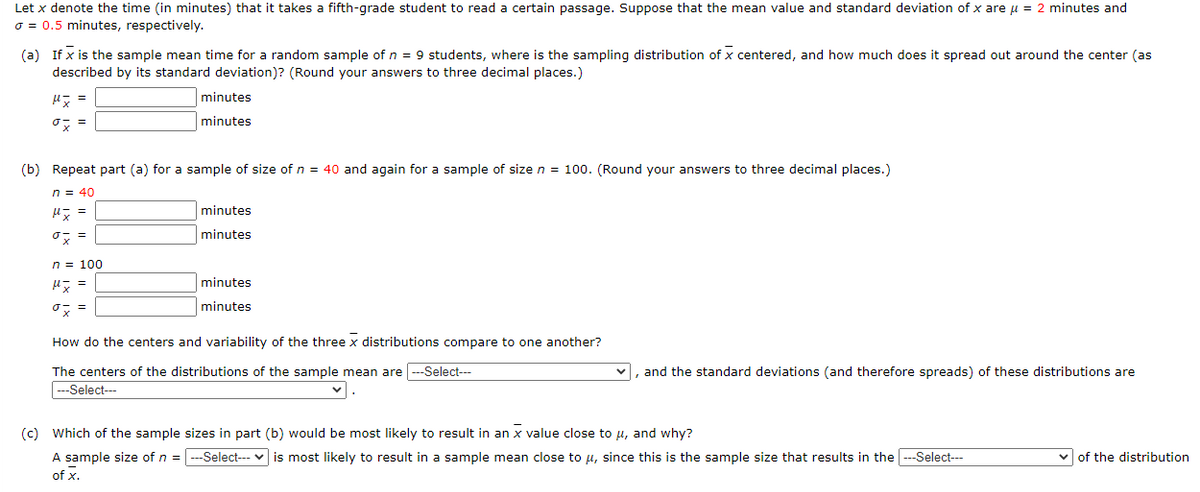
Let x denote the time (in minutes) that it takes a fifth-grade student to read a certain passage. Suppose that the mean value and standard deviation of x are μ = 2 minutes and = 0.5 minutes, respectively. (a) Ifx is the sample mean time for a random sample of n = 9 students, where is the sampling distribution of x centered, and how much does it spread out around the center (as described by its standard deviation)? (Round your answers to three decimal places.) Hx= σx = minutes minutes (b) Repeat part (a) for a sample of size of n = 40 and again for a sample of size n = 100. (Round your answers to three decimal places.) n = 40 μx = o x = n = 100 μx = ox= minutes minutes minutes minutes How do the centers and variability of the three x distributions compare to one another? The centers of the distributions of the sample mean are ---Select--- ---Select--- and the standard deviations (and therefore spreads) of these distributions are (c) Which of the sample sizes in part (b) would be most likely to result in an x value close to μ, and why? A sample size of n = ---Select--- is most likely to result in a sample mean close to μ, since this is the sample size that results in the ---Select--- of x. ✓of the distribution

An SRS of 25 recent birth records at the local hospital was selected. In the sample, the average birth weight was x = 119.6 ounce Suppose the standard deviation is known to bes = 6.5 ounces. Assume that in the population of all babies born in this hospital, the birth weights follow a Normal distribution, with mean m. Based on the 25 recent birth records, the sampling distribution of the sample mean x can be represented by: a. N(119.6, 1.30). b. N(119.6, 6.5). O c. N(m, 1.30). O d. N(m, 6.5).

A fitness center bought a new exercise machine called the Mountain Climber. They decided to keep track of how many people used the machine over a 3-hour period. Here X is the number of people who used the machine.     X 0 1 2 3 4 PX 0.2 0.2 0.1 0.4 0.1 Find the mean,variance and standard deviation

Today, the waves are crashing onto the beach every 5.3 seconds. The times from when a person arrives at the shoreline until a crashing wave is observed follows a Uniform distribution from 0 to 5.3 seconds. Round to 4 decimal places where possible. a. The mean of this distribution is b. The standard deviation is c. The probability that wave will crash onto the beach exactly 3.3 seconds after the person arrives is P(x = 3.3) = d. The probability that the wave will crash onto the beach between 1.9 and 2.3 seconds after the person arrives is P(1.9 3.26) = f. Find the minimum for the upper quartile. seconds.