
MATLAB: An Introduction with Applications
6th Edition
ISBN: 9781119256830
Author: Amos Gilat
Publisher: John Wiley & Sons Inc
expand_more
expand_more
format_list_bulleted
Related questions
Question
all parts please
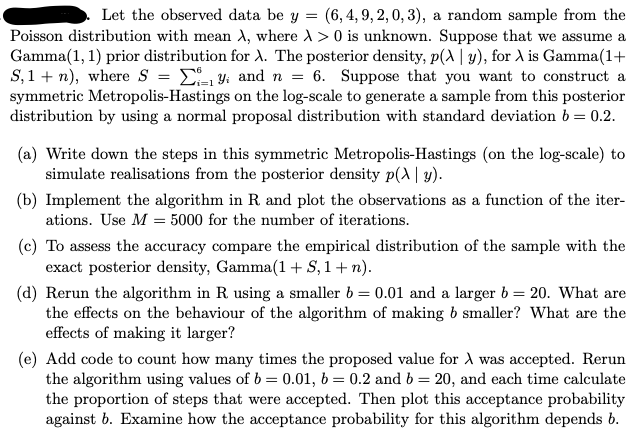

Transcribed Image Text:Let the observed data be y = (6, 4, 9, 2, 0, 3), a random sample from the
Poisson distribution with mean A, where A> 0 is unknown. Suppose that we assume a
Gamma(1, 1) prior distribution for A. The posterior density, p(A | y), for A is Gamma(1+
S, 1 + n), where S = ₁₁y₁ and n = 6. Suppose that you want to construct a
symmetric Metropolis-Hastings on the log-scale to generate a sample from this posterior
distribution by using a normal proposal distribution with standard deviation b = 0.2.
(a) Write down the steps in this symmetric Metropolis-Hastings (on the log-scale) to
simulate realisations from the posterior density p(x|y).
(b) Implement the algorithm in R. and plot the observations as a function of the iter-
ations. Use M = 5000 for the number of iterations.
(c) To assess the accuracy compare the empirical distribution of the sample with the
exact posterior density, Gamma(1 + S, 1 + n).
(d) Rerun the algorithm in R using a smaller b = 0.01 and a larger b = 20. What are
the effects on the behaviour of the algorithm of making b smaller? What are the
effects of making it larger?
(e) Add code to count how many times the proposed value for À was accepted. Rerun
the algorithm using values of b = 0.01, b = 0.2 and b = 20, and each time calculate
the proportion of steps that were accepted. Then plot this acceptance probability
against b. Examine how the acceptance probability for this algorithm depends b.
Expert Solution
This question has been solved!
Explore an expertly crafted, step-by-step solution for a thorough understanding of key concepts.
Step 1: Given information
VIEW Step 2: (a) Writing the steps to simulate the steps in the symmetric Metropolis-Hastings on the log scale
VIEW Step 3: (b) Implementing the algorithm using R
VIEW Step 4: (c) Comparison of the empirical distribution of the sample with the exact posterior density
VIEW Step 5: (d) Running Metropolis Hastings algorithm with different proposal standard deviations
VIEW Step 6: (e) Analysis of acceptance probability in Metropolis Hastings algorithm across different proposals
VIEW Solution
VIEW 
Step by stepSolved in 7 steps with 36 images

Knowledge Booster

Similar questions
- Translatearrow_forwardWilbur landed his plane,arrow_forwardConsider the following loops on the Klein bottle. (1) Decide whether they are orientation reversing or preserving. Explain. (2) In each of the three case, cut the surface by the curve. What is the resulting surface for each case?arrow_forward
arrow_back_ios
SEE MORE QUESTIONS
arrow_forward_ios
Recommended textbooks for you
- MATLAB: An Introduction with ApplicationsStatisticsISBN:9781119256830Author:Amos GilatPublisher:John Wiley & Sons Inc
 Probability and Statistics for Engineering and th...StatisticsISBN:9781305251809Author:Jay L. DevorePublisher:Cengage Learning
 Statistics for The Behavioral Sciences (MindTap C...StatisticsISBN:9781305504912Author:Frederick J Gravetter, Larry B. WallnauPublisher:Cengage Learning
  Elementary Statistics: Picturing the World (7th E...StatisticsISBN:9780134683416Author:Ron Larson, Betsy FarberPublisher:PEARSON
 The Basic Practice of StatisticsStatisticsISBN:9781319042578Author:David S. Moore, William I. Notz, Michael A. FlignerPublisher:W. H. Freeman
 Introduction to the Practice of StatisticsStatisticsISBN:9781319013387Author:David S. Moore, George P. McCabe, Bruce A. CraigPublisher:W. H. Freeman
MATLAB: An Introduction with Applications
Statistics
ISBN:9781119256830
Author:Amos Gilat
Publisher:John Wiley & Sons Inc
Probability and Statistics for Engineering and th...
Statistics
ISBN:9781305251809
Author:Jay L. Devore
Publisher:Cengage Learning
Statistics for The Behavioral Sciences (MindTap C...
Statistics
ISBN:9781305504912
Author:Frederick J Gravetter, Larry B. Wallnau
Publisher:Cengage Learning
Elementary Statistics: Picturing the World (7th E...
Statistics
ISBN:9780134683416
Author:Ron Larson, Betsy Farber
Publisher:PEARSON
The Basic Practice of Statistics
Statistics
ISBN:9781319042578
Author:David S. Moore, William I. Notz, Michael A. Fligner
Publisher:W. H. Freeman
Introduction to the Practice of Statistics
Statistics
ISBN:9781319013387
Author:David S. Moore, George P. McCabe, Bruce A. Craig
Publisher:W. H. Freeman