In crash tests at five miles per hour, the mean bumper repair cost for 15 small cars is 576 dollars with a standard deviation of 186 dollars. In similar test of 21 midsize cars, the mean bumper repair cost is 700 dollars with a standard deviation of 257 dollars. Conduct a hypothesis test based on this sample data, with a = 1%. Answer the question, is the mean bumper repair cost less for small cars than it is for midsize cars?

Hey there! Thank you for posting the question. 

Since you have posted a question with multiple sub-parts, we will solve first three sub-parts for you.

To get remaining sub-part solved please repost the complete question and mention the sub-parts to be solved.

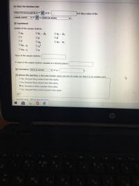
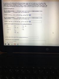
Here we are given that in crash tests at five miles per hour, the mean bumper repair cost for 15 small cars is 576 dollars with a standard deviation of 186 dollars. In similar test of 21 midsize cars, the mean bumper repair cost is 700 dollars  with a standard deviation of 257 dollars. 

That is , 

Sample sizes for small cars and midsize cars is ,

n1 = 15.

n2 = 21.

Sample means for small cars and midsize cars is , 

x̅₁ = 576 dollars.

x̅₂ = 700 dollars.

Sample standard deviations for small cars and midsize cars is , 

s₁ = 186 dollars.

s₂ = 257 dollars.

Given level of significance , α = 1% or 0.01 (in decimal).

It is asked about,

1. State the hypotheses.
2. The correct symbol for the mean of the sampling distribution.
3. The value for the mean of the sampling distribution.

It is asked about hypotheses.

Claim : The mean bumper repair cost is less for small cars than it is for midsized cars.

Null hypotheses : The mean bumper repair cost for small cars is equal to the mean bumper repair cost for for midsize cars.

Symbolically it can be written as , Ho : µ₁ -µ₂ = 0.

Alternative hypotheses : The mean bumper repair cost for small cars is less than the the mean bumper repair cost for for midsize cars.

Symbolically it can be written as , Ho : µ₁ -µ₂ < 0