
Related questions
Concept explainers
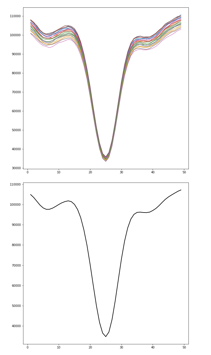
Im trying to plot three plots
1. the actual CCF data in a plot
2. the mean of the CCF data in a plot
3. the residual of the CCF data, which is the CCF data - mean
I have plot 1 and 2 operating okay
import matplotlib.pyplot as plt
import glob
from astropy.io import fits
from astropy.wcs import WCS
import numpy as np
# Step 1: Import the necessary libraries and modules
# Step 2: Create the main figure and axis objects for the initial plot
fig, ax = plt.subplots(figsize=(10, 10))
# Step 3: Get the file paths of FITS files
data_dir = glob.glob('/Users/petrderuyter/Desktop/harpn_sun_release_package_ccf_2018/2018-01-18/*.fits')
# Step 4: Initialize empty lists for storing wavelength and flux data
lams = []
fluxs = []
# Step 5: Read and process each FITS file
for file_path in data_dir:
hdul = fits.open(file_path)
data = hdul[1].data
h1 = hdul[1].header
flux = data[1]
w = WCS(h1, naxis=1, relax=False, fix=False)
lam = w.wcs_pix2world(np.arange(len(flux)), 0)[0]
lams.append(lam)
fluxs.append(flux)
ax.plot(lam, flux)
# Step 6: Calculate the mean flux
mean_ccf = np.mean(fluxs, axis=0)
# Step 7: Create a new figure and axis objects for the second plot (mean data)
fig_mean, ax_mean = plt.subplots(figsize=(10, 10))
# Step 8: Plot the mean data on the second axis
ax_mean.plot(lams[1], mean_ccf, color='k', linewidth=2)
#Calculate the residual
mean_ccf = np.mean(data_dir)
residuals = data_dir - mean_ccf
# Step 9: Customize the plot
ax_mean.set_xlabel('RV [km/s]')
ax_mean.set_ylabel('Normalized CCF')
# Step 10: Set the title and display the plots
plt.title('Mean CCF')
plt.show()
# Step 11: Print the mean flux
print(mean_ccf)
# Plot residuals
plt.plot(residuals, marker='o')
plt.axhline(0, color='red', linestyle='--') # Add a horizontal line at y=0
plt.xlabel('Index')
plt.ylabel('Residual')
plt.title('Residual Plot of CCF Data')
plt.grid(True)
plt.show()


Step by stepSolved in 3 steps


- ram 2: BACK AWAY FROM THE TV! If you sat close enough to an old TV, you could see individual (R)ed, (G)reen and (B)lue (or RGB) “phosphors” that could represent just about any color you could imagine (using “additive color model”). When these three-color components are at their maximum values, the resulting color is white from a distance (which is amazing – look at your screen with a magnifying glass!). When all are off, the color results in black. If red and green are fully on, you’d get a shade of yellow; red and blue on would result in purple, and so on. For computers, each color component is usually represented by one byte (8 bits), and there are 256 different values (0-255) for each. To find the “inverse” of a color (like double-clicking your iFone® button), you subtract the RGB values from 255. The “luminance” (or brightness) of the color = (0.2126*R + 0.7152*G + 0.0722*B). For this program, you need to design (pseudocode) and implement (source code) a Color class that has R, G…arrow_forwardPractice Test Question #1: You want to solve a simplified 4x4 version of the Sudoku game with the following grid configuration (image attached): (a) Show the first ten steps of backtracking search on the sample provided, where you order the variables in increasing order first by row, then by column (in English reading-order), and the values from lowest to highest (1 to 4). Recall that backtracking search uses a depth-first strategy to expand the search tree. (b) Show the first ten steps of backtracking search on this problem with one-step forward checking, with the same variable ordering.arrow_forwardusing python at jupiter lab make a code for image classification and execute itarrow_forward
- Using the MATLAB editor, make a script m-file for the following: The distance an object with constant acceleration has traveled is given by: d = x0 + vt + 0.5at2 And that x0 = 2.25 meters, v = -0.37 meters/sec and a = 0.32 meters/sec2 For values of t from 0 to 45 sec in increments of 3 secMake variables for x0, v and a, and assign valuesFind the values of d in metersDisplay the results on a x-y scatter plot With t the independent variable plotted on the x axisAnd d the dependent variable plotted on the y axisInclude units within the labelsarrow_forwardBy using Karnaugh map, minimize each boolean functions (SOP form) -> If you're uploading pic or image as the answer, please upload it correctly as I was unable to see the answer for this question after it was answered. So I had to post a new question.Thank youarrow_forwardWhat are Contents of PrintArray.asm module.arrow_forward
- Database System ConceptsComputer ScienceISBN:9780078022159Author:Abraham Silberschatz Professor, Henry F. Korth, S. SudarshanPublisher:McGraw-Hill Education
 Starting Out with Python (4th Edition)Computer ScienceISBN:9780134444321Author:Tony GaddisPublisher:PEARSON
 Digital Fundamentals (11th Edition)Computer ScienceISBN:9780132737968Author:Thomas L. FloydPublisher:PEARSON
  C How to Program (8th Edition)Computer ScienceISBN:9780133976892Author:Paul J. Deitel, Harvey DeitelPublisher:PEARSON
 Database Systems: Design, Implementation, & Manag...Computer ScienceISBN:9781337627900Author:Carlos Coronel, Steven MorrisPublisher:Cengage Learning
 Programmable Logic ControllersComputer ScienceISBN:9780073373843Author:Frank D. PetruzellaPublisher:McGraw-Hill Education