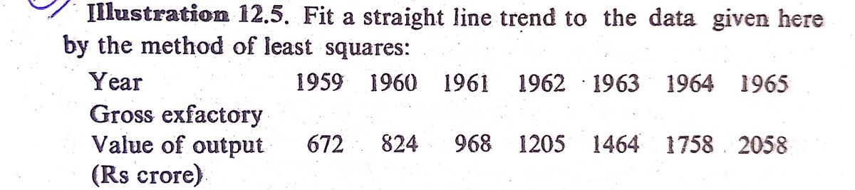
Illustration 12,5. Fit a straight line trend to the data given here by the method of least squares: Year 1959 1960 1961 1962 · 1963 1964 1965 Gross exfactory Value of output (Rş crore) 672 824 968 1205 1464 1758. 2058

The line of best fit through a set of data is ý = 14.714 – 3.985x According to this equation, what is the predicted value of the dependent variable when the independent variable has value 180? Round to 1 decimal place.

The following table gives the data for the grades on the midterm exam and the grades on the final exam. Determine the equation of the regression line, yˆ=b0+b1xy^=b0+b1x. Round the slope and y-intercept to the nearest thousandth. Grades on Midterm and Final Exams Grades on Midterm 78 63 85 92 82 89 69 89 83 61 Grades on Final 77 75 88 92 86 86 80 85 77 63

Before using these mean squares what does we must calculate?

Suppose that a regression yields the following sum of squares: Σ(yi−y¯)^2 = 400, Σ(yi−y^i)^2 = 60, Σ(y^i−y¯)^2 = 340  Then the percentage of the variation in y that is explained by the variation in x is: Answer =  %

Data were collected on the times to recovery (in days) for athletes who had serious concussions. There were two data sets. One data set consisted of the recovery times of 200 athletes who were treated for their concussion and the other data set consisted of the recovery times of 200 athletes who received no treatment for their concussions. The histograms summarize the two data sets. For simplicity call the histogram on the left Figure 1, and the one on the right Figure 2. (a)Researchers claim that those who were not treated for concussion tended to have longer recovery times than those who were treated. According to this claim, which of these two histograms corresponds to the data for those who were not treated? (b) In no more than two sentences, justify your answer to part (a). (c) From Figure 1, find the (approximate) proportion of athletes that recovered in 55 or fewer days. (d) Which measure of centrality would you prefer to use for the data that led to Figure 2: the sample mean or…

The line of best fit through a set of data is y = 41.762 2.926x According to this equation, what is the predicted value of the dependent variable when the independent variable has value 50? y = Round to 1 decimal place.

A patient is classified as having gestational diabetes if their average glucose level is above 140 milligrams per deciliter (mg/dl) one hour after a sugary drink is ingested. Rebecca's doctor is concerned that she may suffer from gestational diabetes. There is variation both in the actual glucose level and in the blood test that measures the level. Rebecca's measured glucose level one hour after ingesting the sugary drink varies according to the Normal distribution with μ=140+5 mg/dl and σ=5+1 mg/dl. Using the Central Limit Theorem, determine the probability of Rebecca being diagnosed with gestational diabetes if her glucose level is measured: Once? n=5+2 times n=5+4 times Comment on the relationship between the probabilities observed in (a), (b), and (c). Explain, using concepts from lecture why this occurs and what it means in context.

This question had 6 parts and I was ask to resend the last 3.  the question is  The line of best fit for a data set is y= 1.1x+3.4. Find the residual for each of the coordinate pairs (x,y).

please only answer the last part "Suppose that real income per capita in New Jersey increases by​ 1% in the next year. Use the results in column​ (4) to predict the change in the number of traffic fatalities in the next year. "