
MATLAB: An Introduction with Applications
6th Edition
ISBN: 9781119256830
Author: Amos Gilat
Publisher: John Wiley & Sons Inc
expand_more
expand_more
format_list_bulleted
Related questions
Question

Transcribed Image Text:Listen
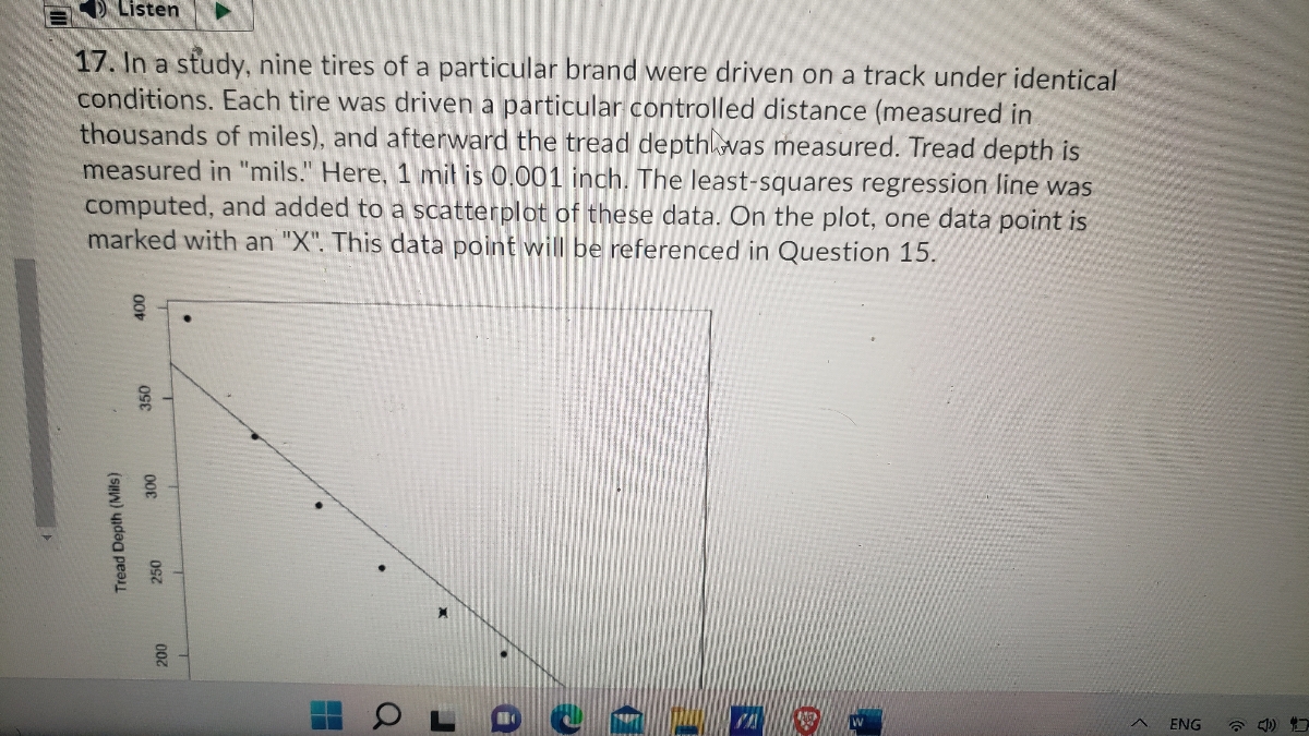
17. In a study, nine tires of a particular brand were driven on a track under identical
conditions. Each tire was driven a particular controlled distance (measured in
thousands of miles), and afterward the tread depthlvas measured. Tread depth is
measured in "mils." Here, 1 mil is 0.001 inch. The least-squares regression line was
computed, and added to a scatterplot of these data. On the plot, one data point is
marked with an "X". This data point will be referenced in Question 15.
ENG
* 4)
Tread Depth (Mils)

Transcribed Image Text:Attempt 1
The equation of the least-squares regression line is:
Tread Depth = 360.64 - 11.39x (thousands of miley)
Also, 2
= 0.953.
Which of the following statements is true?
a) About 95.3% of the variation in tread depth is explained by the regression on miles.
O b) According to the least-squares regression line, the groove depth of a new tire (driven
0 miles) is predicted to be 360.64 mils.
c) According to the least-squares regression line, we would predict a decrease in groove
depth of 11.39 mils for each 1000 miles driven on a tire.
d) All of the above.
Expert Solution
This question has been solved!
Explore an expertly crafted, step-by-step solution for a thorough understanding of key concepts.

This is a popular solution

Trending nowThis is a popular solution!

Step by stepSolved in 2 steps with 2 images

Knowledge Booster

Similar questions
- STER. 1. Wine Consumption. The table below gives the U.S. adult wine consumption, in gallons per person per year, for selected years from 1980 to 2005. a) Create a scatterplot for the data. Graph the scatterplot Year Wine below. Consumption 2.6 b) Determine what type of model is appropriate for the 1980 data. 1985 2.3 c) Use the appropriate regression on your calculator to find a Graph the regression equation in the same coordinate plane below. d) According to your model, in what year was wine consumption at a minimum? A e) Use your model to predict the wine consumption in 2008. 1990 2.0 1995 2.1 2000 2.5 2005 2.8arrow_forwardNonearrow_forwardA simple regression model developed for ten pairs of data resulted in a sum of squares of error, SSE = 125. The standard error of the estimate is 12.5 3.5 25 15.6 O 3.95arrow_forward
- 1. Develop a simple linear regression equation for starting salaries using an independent variable that has the closest relationship with the salaries. Explain how you chose this variable.arrow_forwardAnswer the following: 2. Describe the form, direction, and strength of the relationship between these variables. Does there appear to be any outliers? 3. The equation of least-squares regression line is y = 6.871 + 0.061x. This line goes through the points (0, 6.9) and (700, 49.5). Use these points to add the regression line to your scatterplot above. 4. One animal is farthest from the regression line and is an outlier for these two variables. Find the name of this animal and write a sentence describing how its position differs from the overall relationship among the other animals. 5. The elephant has the longest gestation period of these animals. a. Considering only the gestation variable, would you say that the elephant is an outlier? Write a sentence or two explaining why or why not? b. Considering both variables and the relationship between average life span and average gestation period, would you say the elephant is an outlier now? Write a sentence or two explaining why or why…arrow_forwardFor Data Set 9 in Appendix B, “Bear Measurements,” we get this regression equation: Weight = -274 + 0.426 Length + 12.1 Chest Size, with R2 = 0.928. Interpret the multiple coefficient of determination – what does this value tell us?arrow_forward
- Find the least-squares regression line treating square footage as the explanatory variable. y = (Round the slope to three decimal places as needed. Round the intercept to one decimal place as needed.)arrow_forwardA local retail store compared their monthly sales of umbrellas with the amount of rainfall that occured during that month. They computed the following statistics: Rainfall (in) # of umbrellas mean = 4.64 mean = 34.2 SD = 1.17 SD = 13.2 r = 0.8 1. Find the equation for the regression line that predicts the monthly sales of umbrellas from monthly rainfall.arrow_forwardwhat % of the variation is ( height, or head circumference) explained by the least-squares regression model. (Round to one decimal place as needed.)arrow_forward
arrow_back_ios
arrow_forward_ios
Recommended textbooks for you
- MATLAB: An Introduction with ApplicationsStatisticsISBN:9781119256830Author:Amos GilatPublisher:John Wiley & Sons Inc
 Probability and Statistics for Engineering and th...StatisticsISBN:9781305251809Author:Jay L. DevorePublisher:Cengage Learning
 Statistics for The Behavioral Sciences (MindTap C...StatisticsISBN:9781305504912Author:Frederick J Gravetter, Larry B. WallnauPublisher:Cengage Learning
  Elementary Statistics: Picturing the World (7th E...StatisticsISBN:9780134683416Author:Ron Larson, Betsy FarberPublisher:PEARSON
 The Basic Practice of StatisticsStatisticsISBN:9781319042578Author:David S. Moore, William I. Notz, Michael A. FlignerPublisher:W. H. Freeman
 Introduction to the Practice of StatisticsStatisticsISBN:9781319013387Author:David S. Moore, George P. McCabe, Bruce A. CraigPublisher:W. H. Freeman
MATLAB: An Introduction with Applications
Statistics
ISBN:9781119256830
Author:Amos Gilat
Publisher:John Wiley & Sons Inc
Probability and Statistics for Engineering and th...
Statistics
ISBN:9781305251809
Author:Jay L. Devore
Publisher:Cengage Learning
Statistics for The Behavioral Sciences (MindTap C...
Statistics
ISBN:9781305504912
Author:Frederick J Gravetter, Larry B. Wallnau
Publisher:Cengage Learning
Elementary Statistics: Picturing the World (7th E...
Statistics
ISBN:9780134683416
Author:Ron Larson, Betsy Farber
Publisher:PEARSON
The Basic Practice of Statistics
Statistics
ISBN:9781319042578
Author:David S. Moore, William I. Notz, Michael A. Fligner
Publisher:W. H. Freeman
Introduction to the Practice of Statistics
Statistics
ISBN:9781319013387
Author:David S. Moore, George P. McCabe, Bruce A. Craig
Publisher:W. H. Freeman