
MATLAB: An Introduction with Applications
6th Edition
ISBN: 9781119256830
Author: Amos Gilat
Publisher: John Wiley & Sons Inc
expand_more
expand_more
format_list_bulleted
Related questions
Question
thumb_up100%
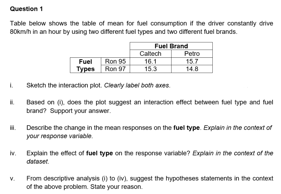

Transcribed Image Text:Question 1
Table below shows the table of mean for fuel consumption if the driver constantly drive
80km/h in an hour by using two different fuel types and two different fuel brands.
Fuel Brand
iii.
iv.
V.
Fuel
Types
Ron 95
Ron 97
Caltech
16.1
15.3
Petro
15.7
14.8
Sketch the interaction plot. Clearly label both axes.
Based on (i), does the plot suggest an interaction effect between fuel type and fuel
brand? Support your answer.
Describe the change in the mean responses on the fuel type. Explain in the context of
your response variable.
Explain the effect of fuel type on the response variable? Explain in the context of the
dataset.
From descriptive analysis (i) to (iv), suggest the hypotheses statements in the context
of the above problem. State your reason.
Expert Solution
This question has been solved!
Explore an expertly crafted, step-by-step solution for a thorough understanding of key concepts.

Step by stepSolved in 2 steps with 1 images

Knowledge Booster

Similar questions
- Prices and mileage of 44 Toyota Prius cars. Prices ranged from $17,043 to $48,935. Mileage ranged from 403 to 70,838. While I did not share the cars were 2017 to 2020 models. Please show all work. Create a scatter plot of prices (Y) and mileage (X). What interpretation can you make using this scatter plot? Does this model meet the Linearity assumption? Provide evidence and a discussion of support for meeting the assumption. Does this model meet the Independent Errors assumption? Provide evidence and a discussion of support for meeting the assumption. Price Mileage 17167 67380 24500 8137 20700 14907 20700 13906 18995 39268 21985 3292 19995 32630 19983 36074 19477 35484 20980 23954 24940 7001 24940 7991 25480 3476 17960 41051 25980 403 24500 8137 18588 66109 18788 51022 19200 32753 21985 38838 24512 2307 22997 33671 18480 27233 18480 27758 17043 70838 17761 21967 18488 11686 17793 26080 17900 36655 18100 46264…arrow_forwardHi! I need help finding the answers in the yellow boxes please :) Thank you so so much!!arrow_forwardComplete parts (a) through (h) for the data below. X 2 3 4 6 7 y 3 6 10 15 18 (a) By hand, draw a scatter diagram treating x as the explanatory variable and y as the response variable. Choose the correct scatter diagram below. A. Ax 10- 20 y 20- Ay 10 10- (b) Find the equation of the line containing the points (2,3) and (7,18). y= ☐ X X+ (Type integers or simplified fractions.) X 20 -0 10 Xarrow_forward
- The table below shows the number of state-registered automatic weapons and the murder rate for several Northwestern states. 11.6 8.1 7.1 3.9 2.9 2.6 2.1 0.7 13.7 10.7 10.2 7 6.5 6.5 5.7 4.7 thousands of automatic weapons y = murders per 100,000 residents This data can be modeled by the linear equation 0.83x + 4.08 a. How many murders per 100,000 residents can be expected in a state with 10.3 thousand automatic weapons? Round to 3 decimal places. murders per 100,000 residents b. How many murders per 100,000 residents can be expected in a state with 2.5 thousand automatic weapons? Round to 3 decimal places. murders per 100,000 residentsarrow_forwardThe graph plots the gas mileage of various cars from the same model year versus the weight of these cars in thousands of pounds. Describe the association between the two variables. Also explain what the point at the very top represents. 3.75 Weight (thousands of pounds) BIUA A LE xx, E 12pt Paragraph Submarrow_forwardNeed helparrow_forward
- I can do the scatter plot diagram I just need help With identifying the Y axis and the X access and the Form directions strength And outlierarrow_forwardThe basic hypothesis is that people who play sports are more likely than others to watch sport on TV. Your first task is to crosstabulate the data involving the playing and watching of sports and to determine the direction and strength of that relationship. Write out your findings about this basic relationship. Your next task is to determine the direction and strength of the partial relationships when you control for the gender of individuals.arrow_forwardGiven the data as shown in the table below X Y 2 12 10 4 10 Use technology to graph the scatterplot and the best-fit line of the data. Find your corect graph belowarrow_forward
arrow_back_ios
arrow_forward_ios
Recommended textbooks for you
- MATLAB: An Introduction with ApplicationsStatisticsISBN:9781119256830Author:Amos GilatPublisher:John Wiley & Sons Inc
 Probability and Statistics for Engineering and th...StatisticsISBN:9781305251809Author:Jay L. DevorePublisher:Cengage Learning
 Statistics for The Behavioral Sciences (MindTap C...StatisticsISBN:9781305504912Author:Frederick J Gravetter, Larry B. WallnauPublisher:Cengage Learning
  Elementary Statistics: Picturing the World (7th E...StatisticsISBN:9780134683416Author:Ron Larson, Betsy FarberPublisher:PEARSON
 The Basic Practice of StatisticsStatisticsISBN:9781319042578Author:David S. Moore, William I. Notz, Michael A. FlignerPublisher:W. H. Freeman
 Introduction to the Practice of StatisticsStatisticsISBN:9781319013387Author:David S. Moore, George P. McCabe, Bruce A. CraigPublisher:W. H. Freeman
MATLAB: An Introduction with Applications
Statistics
ISBN:9781119256830
Author:Amos Gilat
Publisher:John Wiley & Sons Inc
Probability and Statistics for Engineering and th...
Statistics
ISBN:9781305251809
Author:Jay L. Devore
Publisher:Cengage Learning
Statistics for The Behavioral Sciences (MindTap C...
Statistics
ISBN:9781305504912
Author:Frederick J Gravetter, Larry B. Wallnau
Publisher:Cengage Learning
Elementary Statistics: Picturing the World (7th E...
Statistics
ISBN:9780134683416
Author:Ron Larson, Betsy Farber
Publisher:PEARSON
The Basic Practice of Statistics
Statistics
ISBN:9781319042578
Author:David S. Moore, William I. Notz, Michael A. Fligner
Publisher:W. H. Freeman
Introduction to the Practice of Statistics
Statistics
ISBN:9781319013387
Author:David S. Moore, George P. McCabe, Bruce A. Craig
Publisher:W. H. Freeman