If the level of employee satisfaction drops below 0.60 overall, then there is a belief that there may be a serious problem with morale in that department. There have been rumors that the Human Resources department (hr in the data file) may be having just such issues. Using a statistical package, test to determine if the mean employee satisfaction level in the Human Resources department is less than 0.60. 1. Is satisfaction level a qualitative or quantitative variable? 2. Graph the employee satisfaction level for the Human Resources department with an appropriate graph and calculate statistics appropriate for this type of data. 3. Conduct the appropriate hypothesis test using the following steps. a. Determine the null and alternative hypotheses. b. Use a significance level of a = 0.05. c. Validate the assumptions of the hypothesis test, identify the appropriate test statistic, and compute its value. d. Determine the P-value. e. Make a decision to reject or fail to reject the null hypothesis, H f. State the conclusion in terms of the original problem. 4. Based on our conclusion from the previous step, what type of error could we have just made (Type I or Type II)? State the practical implications of this error. 5. Would it be appropriate to compare this test to a confidence interval for the mean? Why or why not?

MATLAB: An Introduction with Applications

6th Edition

ISBN:9781119256830

Author:Amos Gilat

Publisher:Amos Gilat

Chapter1: Starting With Matlab

Section: Chapter Questions

Problem 1P

See similar textbooks

Related questions

Question

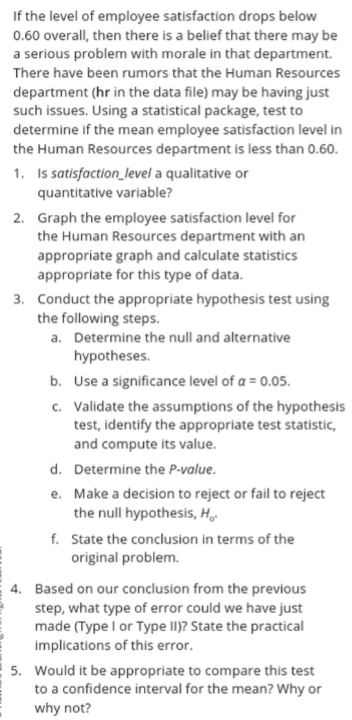
If the level of employee satisfaction drops below
0.60 overall, then there is a belief that there may be
a serious problem with morale in that department.
There have been rumors that the Human Resources
department (hr in the data file) may be having just
such issues. Using a statistical package, test to
determine if the mean employee satisfaction level in
the Human Resources department is less than 0.60.
1. Is satisfaction level a qualitative or
quantitative variable?
2. Graph the employee satisfaction level for
the Human Resources department with an
appropriate graph and calculate statistics
appropriate for this type of data.
3. Conduct the appropriate hypothesis test using
the following steps.
a. Determine the null and alternative
hypotheses.
b. Use a significance level of a = 0.05.
c. Validate the assumptions of the hypothesis
test, identify the appropriate test statistic,
and compute its value.
d. Determine the P-value.
e.
Make a decision to reject or fail to reject
the null hypothesis, H.
f. State the conclusion in terms of the
original problem.
4. Based on our conclusion from the previous
step, what type of error could we have just
made (Type I or Type II)? State the practical
implications of this error.
5. Would it be appropriate to compare this test
to a confidence interval for the mean? Why or
why not?

Expert Solution

Trending now

This is a popular solution!

Step by step

Solved in 3 steps with 3 images

SEE SOLUTION Check out a sample Q&A here

Follow-up Questions

Read through expert solutions to related follow-up questions below.

Follow-up Question

I still don't get how to make the chart. Here is the data I was given for satisfaction

satisfaction_level
0.78
0.8
0.72
0.67
0.81
0.92
0.89
0.52
0.45
0.84
0.81
0.75
0.78
0.75
0.76
0.11
0.78
0.76
0.74
0.89
0.82
0.74
0.71
0.68
0.75
0.74
0.75
0.84
0.71
0.78
0.75
0.71
0.81
0.87
0.75
0.74
0.79
0.84
0.84
0.57
0.94
0.43
0.93
0.44
0.88
0.89
0.87
0.91
0.81
0.68
0.85
0.85
0.81
0.73
0.9
0.76
0.73
0.74
0.75
0.89
0.81
0.81
0.84
0.83
0.89
0.85
0.78
0.79
0.84
0.84
0.87
0.71
0.74
0.89
0.82
0.86
0.89
0.87
0.81
0.81
0.91
0.9
0.88
0.86
0.82
0.89
0.83
0.84
0.91
0.44
0.71
0.74
0.63
0.69
0.83
0.9
0.84
0.77
0.86
0.71
0.77
0.74
0.74
0.74
0.75
0.81
0.46
0.81
0.88
0.7
0.89
0.37
0.81
0.88
0.89
0.84
0.36
0.31
0.81
0.82
0.74
0.73
0.89
0.45
0.11
0.37
0.84
0.41
0.76
0.11
0.84
0.39
0.11
0.45
0.37
0.4
0.39
0.11
0.83
0.11
0.39
0.45
0.1
0.9
0.45
0.79
0.9
0.11
0.43
0.31
0.32
0.45
0.81
0.41
0.11
0.1
0.7
0.54
0.41
0.38
0.37
0.11
0.4
0.1
0.89
0.11
0.36
0.4
0.09
0.4
0.37
0.44
0.09
0.92
0.74
0.09
0.89
0.09
0.27
0.1
0.1
0.77
0.9
0.39
0.76
0.1
0.87
0.38
0.77
0.78
0.44
0.38
0.43
0.39
0.88
0.45
0.4
0.36
0.36
0.9
0.43
0.89
0.1
0.37
0.37
0.87
0.4
0.9
0.37
0.44
0.85
0.78
0.42
0.92
0.11
0.42
0.48
0.83
0.94
0.93
0.93
0.91
0.91
0.97
0.98
0.94
0.89
0.95
0.97
0.96
0.87
0.91
0.79
0.79
0.99
0.87
0.96
0.94
0.91
0.92
0.88
0.91
0.96
0.82
0.94
0.91
0.92
0.84
0.91
0.95
0.98
0.98
0.94
0.91
0.81
0.99
0.91
0.81
0.91
0.74
0.99
0.82
0.91
0.97
0.83
0.91
0.98
0.94
0.91
0.91
0.92
0.96
0.94
0.87
0.91
0.91
0.91
0.98
0.99
0.94
0.95
0.94
0.45
0.92
0.91
0.97
0.89
0.45
0.37
0.91
0.41
0.91
0.91
0.91
0.4
0.41
0.91
0.73
0.43
0.87
0.11
0.4
0.41
0.82
0.61
0.11
0.37
0.41
0.37
0.88
0.1
0.44
0.38
0.11
0.09
0.45
0.1
0.45
0.77
0.44
0.39
0.81
0.89
0.37
0.9
0.41
0.37
0.61
0.81
0.71
0.81
0.4
0.09
0.48
0.91
0.43
0.33
0.41
0.41
0.37
0.31
0.09
0.1
0.76
0.41
0.72
0.4
0.91
0.1
0.4
0.82
0.1
0.37
0.36
0.39
0.36
0.86
0.73
0.56
0.44
0.31
0.77
0.44
0.38
0.45
0.38
0.36
0.75
0.1
0.1
0.45
0.42
0.78
0.45
0.84
0.11
0.42
0.45
0.46
0.09
0.87
0.1
0.91
0.76
0.74
0.92
0.76
0.47
0.73
0.09
0.91
0.82
0.28
0.84
0.45
0.45
0.91
0.42
0.82
0.11
0.42
0.82
0.09
0.1
0.86
0.4
0.45
0.42
0.74
0.55
0.37
0.41
0.89
0.41
0.44
0.87
0.1
0.41
0.11
0.43
0.77
0.41
0.41
0.36
0.77
0.81
0.39
0.09
0.44
0.1
0.36
0.81
0.81
0.85
0.1
0.37
0.09
0.44
0.86
0.77
0.41
0.4
0.43
0.43
0.8
0.8
0.82
0.37
0.37
0.09
0.9
0.41
0.1
0.44
0.89
0.42
0.87
0.45
0.11
0.09
0.76
0.11
0.37
0.1
0.77
0.42
0.38
0.32
0.38
0.19
0.1
0.76
0.53
0.39
0.11
0.1
0.84
0.82
0.1
0.59
0.44
0.89
0.91
0.66
0.11
0.43
0.78
0.11
0.83
0.39
0.38
0.37
0.44
0.53
0.09
0.11
0.83
0.88
0.1
0.09
0.44
0.39
0.87
0.74
0.1
0.74
0.75
0.41
0.41
0.09
0.09
0.39
0.4
0.37
0.1
0.43
0.75
0.37
0.11
0.45
0.87
0.11
0.45
0.81
0.77
0.89
0.43
0.78
0.37
0.37
0.85
0.41
0.11
0.75
0.82
0.79
0.43
0.1
0.46
0.43
0.43
0.11
0.09
0.37
0.4
0.1
0.41
0.79
0.11
0.1
0.44
0.25
0.44
0.73
0.75
0.36
0.37
0.39
0.48
0.57
0.9
0.39
0.44
0.81
0.74
0.44
0.41
0.4
0.46
0.8
0.87
0.39
0.38
0.66
0.1
0.37
0.1
0.09
0.86
0.11
0.37
0.11
0.77
0.84
0.1
0.83
0.11
0.86
0.38
0.11
0.45
0.1
0.09
0.39
0.37
0.81
0.09
0.1
0.39
0.83
0.45
0.43
0.8
0.1
0.1
0.36
0.38
0.78
0.44
0.41
0.72
0.46
0.1
0.34
0.11
0.38
0.82
0.39
0.44
0.43
0.84
0.43
0.37
0.74
0.73
0.37
0.58
0.4
0.51
0.46
0.45
0.46
0.39
0.09
0.09
0.37
0.1
0.77
0.79
0.43
0.38
0.77
0.44
0.39
0.78
0.1
0.1
0.75
0.46
0.91
0.1
0.72
0.11
0.11
0.46
0.37
0.46
0.43
0.11
0.73
0.43
0.86
0.1
0.4
0.11
0.86
0.42
0.79
0.1
0.09
0.09
0.87
0.36
0.42
0.84
0.1
0.78
0.35
0.1
0.11
0.43
0.38
0.46
0.89
0.45
0.44
0.74
0.45
0.79
0.79
0.11
0.42
0.64
0.4
0.84
0.73
0.4
0.36
0.43
0.11
0.91
0.8
0.42
0.31
0.44
0.38
0.45
0.43
0.45
0.43
0.43
0.09
0.43
0.79
0.85
0.38
0.11
0.83
0.81
0.42
0.11
0.11
0.1
0.5
0.44
0.11
0.39
0.11
0.36
0.43
0.4
0.86
0.38
0.46
0.37
0.43
0.66
0.37
0.77
0.88
0.89
0.81
0.81
0.89
0.81
0.39
0.83
0.89
0.75
0.84
0.81
0.82
0.81
0.81
0.81
0.82
0.88
0.39
0.67
0.71
0.81
0.44
0.91
0.72
0.76
0.44
0.85
0.78
0.39
0.78
0.91
0.91
0.71
0.83
0.75
0.93
0.81
0.43
0.91
0.43
0.85
0.91
0.81
0.76
0.45
0.86
0.71
0.11
0.84
0.79
0.38
0.8
0.84
0.89
0.75
0.74
0.41
0.44
0.37
0.11
0.87
0.59
0.38
0.72
0.73
0.39
0.89
0.89
0.91
0.43
0.81
0.37
0.66
0.79
0.44
0.79
0.91
0.54
0.37
0.37
0.82
0.45
0.79
0.42
0.74
0.79
0.93
0.81
0.39
0.91
0.82
0.81
0.42
0.74
0.38
0.39
0.87
0.78
0.84
0.81
0.91
0.89
0.82
0.38
0.89
0.87
0.88
0.78
0.81
0.81
0.43
0.75
0.74
0.85
0.73
0.84
0.78
0.83
0.83
0.45
0.76
0.92
0.92
0.79
0.83
0.8
0.44
0.89
0.48
0.38
0.82
0.37
0.4
0.83
0.84
0.82
0.81
0.78
0.46
0.77
0.83
0.9
0.72
0.74
0.92
0.73
0.81
0.71
0.87
0.67
0.69
0.61
0.71
0.74
0.71
0.46
0.69
0.81
0.79
0.73
0.71
0.37
0.38
0.8
0.79
0.85
0.72
0.71
0.88
0.72
0.76
0.92
0.71
0.39
0.71
0.45
0.44
0.85
0.83
0.75
0.81
0.76
0.74
0.74
0.79
0.76
0.85
0.84
0.68
0.78
0.7
0.86
0.87
0.81
0.81
0.85
0.91
0.76
0.74
0.92
0.76
0.76
0.73
0.83
0.88

Solution

by Bartleby Expert

SEE SOLUTION

Follow-up Question

What program did you use to type in your code to create the graph?

Solution

by Bartleby Expert

SEE SOLUTION