ht then click on format trendline.4.Click on linear and choose line of equation and R2 val ue.5.Then ok.Solution:Here we have to find the equation of line and graph.So we get ap propriate graph and the equation of line using excel.Steps: 1.Enter x and y values in exce I sheet.2.Select x and y values and click on insert then click on scatter plot.3.Click on any point on the graph click right then click on format trendline.4.Click on linear and choose line of equation and R2 value.5.Then ok. 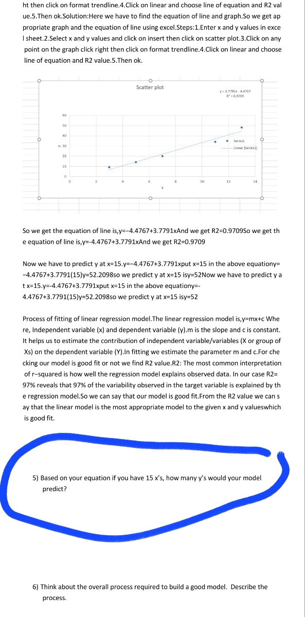NO 40 94 20 10 0 Scatter plot -3.7791x 4476? ²-0,9709 . 12 Serial Linear Berest) 34 So we get the equation of line is,y=-4.4767+3.7791xAnd we get R2=0.9709So we get th e equation of line is,y=-4.4767+3.7791xAnd we get R2=0.9709 Now we have to predict y at x=15.y=-4.4767+3.7791xput x=15 in the above equationy= -4.4767+3.7791(15)y=52.2098so we predict y at x=15 isy=52Now we have to predict y a tx=15.y=-4.4767+3.7791xput x=15 in the above equationy=- 4.4767+3.7791(15)y=52.2098so we predict y at x=15 isy=52 Process of fitting of linear regression model. The linear regression model is,y=mx+c Whe re, Independent variable (x) and dependent variable (y).m is the slope and c is constant. It helps us to estimate the contribution of independent variable/variables (X or group of Xs) on the dependent variable (Y).In fitting we estimate the parameter m and c.For che cking our model is good fit or not we find R2 value.R2: The most common interpretation of r-squared is how well the regression model explains observed data. In our case R2= 97% reveals that 97% of the variability observed in the target variable is explained by th e regression model. So we can say that our model is good fit.From the R2 value we can s ay that the linear model is the most appropriate model to the given x and y valueswhich is good fit. 5) Based on your equation if you have 15 x's, how many y's would your model predict? 6) Think about the overall process required to build a good model. Describe the process.

Write an equation for the line through the point (2, - 3) that... A. is vertical B. is horizontal 1 C. Has slope 2 D. also passes through the point ( – 5, - 4): E. is perpendicular to the line -4x +y = 2: %3D > Next Question

A survey was distributed to a group of people asking them how many times they had ordered takeout in the past week. They were also asked how much money they saved that week. The scatter plot displays the relationship between the data collected.  the trend line goes through the points (1,230) and (3,190). What is the equation of the trend line. The equation should be in slope form.  interpret the slope and y intercept in this context.  predict the amount of money a person save when they order takeout 9 times.

Please do step by step so i can be able to understand?