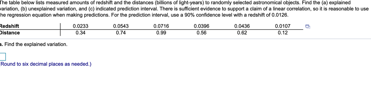
he table below lists measured amounts of redshift and the distances (billions of light-years) to randomly selected astronomical objects. Find the (a) explained ariation, (b) unexplained variation, and (c) indicated prediction interval. There is sufficient evidence to support a claim of a linear correlation, so it is reasonable to use he regression equation when making predictions. For the prediction interval, use a 90% confidence level with a redshift of 0.0126.

The table below lists measured amounts of redshift and the distances (billions of light-years) to randomly selected astronomical objects. Find the (a) explained variation, (b) unexplained variation, and (c) indicated prediction interval. There is sufficient evidence to support a claim of a linear correlation, so it is reasonable to use the regression equation when making predictions. For the prediction interval, use a 90% confidence level with a redshift of 0.0126. Redshift Distance 0.0238 0.31 a. Find the explained variation. 0.0543 0.74 (Round to six decimal places as needed.) b. Find the unexplained variation. (Round to six decimal places as needed.) c. Find the indicated prediction interval. 0.0722 1.02 billion light-years

Heights (cm) and weights (kg) are measured for 100 randomly selected adult males, and range from heights of 138 to 188 cm and weights of 40 to 150 kg. Let the predictor variable x be the first variable given. The 100 paired measurements yield x = 167.61 cm, y = 81.52 kg, r=0.271, P-value=0.006, and y = -103 +1.18x. Find the best predicted value of ŷ (weight) given an adult male who is 155 cm tall. Use a 0.10 significance level. The best predicted value of y for an adult male who is 155 cm tall is (Round to two decimal places as needed.) kg.

The mean exam score for 44. male high school students are 19.9 and the population standard deviation is 5.2. The mean exam score for 55female high school students is 19.4 and the population standard deviation is 4.9. At α=0.01​, can you reject the claim that male and female high school students have equal exam​ scores? Complete parts​ (a) through​ (e).   ​(a) Identify the claim and state H0 and Ha.   What is the​ claim?   A. Male high school students have lower exam scores than female students.   B. Male and female high school students have different exam scores.   C. Male and female high school students have equal exam scores.   D. Male high school students have greater exam scores than female students.   What are H0 and Ha​?   Find the critical​ value(s) and identify the rejection​ region(s). The critical​ value(s) is/are   Find the standardized test statistic z for μ1−μ2.

Heights (cm) and weights (kg) are measured for 100 randomly selected adult males, and range from heights of 132 to 193 cm and weights of 39 to 150 kg. Let the predictor variable x be the first variable given. The 100 paired measurements yield x = 167.59 cm, y = 81.52 kg, r= 0.416, P-value = 0.000, and y = - 102 + 1.13x. Find the best predicted value of y (weight) given an adult male who is 147 cm tall. Use a 0.05 significance level. The best predicted value of y for an adult male who is 147 cm tall is kg. (Round to two decimal places as needed.)

Heights (cm) and weights (kg) are measured for 100 randomly selected adult males, and range from heights of 137 to 189 cm and weights of 37 to 150 kg. Let the predictor variable x be the first variable given. The 100 paired measurements yield x = 167.50 cm, y =81.41 kg, r=0.232, P-value = 0.020, and y = - 109 + 1.17x. Find the best predicted value of y (weight) given an adult male who is 145 cm tall. Use a 0.01 significance level. The best predicted value of y for an adult male who is 145 cm tall is kg. (Round to two decimal places as needed.)

Heights (cm) and weights (kg) are measured for 100 randomly selected adult males, and range from heights of 137 to 192 cm and weights of 40 to 150 kg. Let the predictor variable x be the first variable given. The 100 paired measurements yield x = 167.80 cm, y = 81.45 kg, r=0.211, P-value = 0.035, and y = -103 +1.07x. Find the best predicted value of ŷ (weight) given an adult male who is 145 cm tall. Use a 0.01 significance level. The best predicted value of y for an adult male who is 145 cm tall is (Round to two decimal places as needed.) kg.

Heights (cm) and weights (kg) are measured for 100 randomly selected adult males, and range from heights of 138 to 190 cm and weights of 40 to 150 kg. Let the predictor variable x be the first variable given. The 100 paired measurements yield x = 167.88 cm, y = 81.51 kg, r=0.195, P-value = 0.052, and y= - 105 + 1.05x. Find the best predicted value of y (weight) given an adult male who is 184 cm tall. Use a 0.01 significance level. The best predicted value of y for an adult male who is 184 cm tall is kg. (Round to two decimal places as needed.)

Heights (cm) and weights (kg) are measured for 100 randomly selected adult males, and range from heights of 135 to 191 cm and weights of 39 to 150 kg. Let the predictor variable x be the first variable given. The 100 paired measurements yield x = 167.76 cm, y = 81.33 kg, r= 0.212, P-value = 0.034, and y = - 105+ 1.03x. Find the best predicted value of y (weight) given an adult male who is 139 cm tall. Use a 0.10 significance level. The best predicted value of y for an adult male who is 139 cm tall is kg (Round to two decimal places as needed.)

Consider the following information about variable X: Mean = 4, standard deviation = 2. Consider the following information about variable Y: Mean = 5, standard deviation = 3. If there is a correlation of r = 0.52 between variable X and variable Y, what is the intercept for a simple linear regression equation predicting Y on the basis of X?  Please provide your answer as a raw score (not a z score) with a minimum of two decimal places.