
Big Ideas Math A Bridge To Success Algebra 1: Student Edition 2015
1st Edition
ISBN: 9781680331141
Author: HOUGHTON MIFFLIN HARCOURT
Publisher: Houghton Mifflin Harcourt
expand_more
expand_more
format_list_bulleted
Related questions
Question
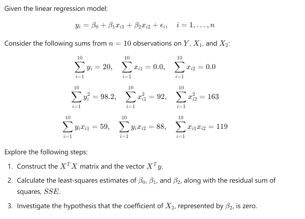

Transcribed Image Text:Given the linear regression model:
Yi = Bo+B1x1 + ẞ2xi2 + Єi,
i = 1,..., n
Consider the following sums from n = 10 observations on Y, X1, and X2:
10
10
10
Σ3 = 20, Σ
i=1
10
Συ? = 98.2,
i=1
i=1
10
10
10
71 =0.0, Σ
i=1
10
x12 = 0.0
Σαμ = 92, Σα?
i=1
= 163
i=1
10
Σ Yixil
=
59, Yixi2 = 88,
Xi1i2=119
i=1
i=1
i=1
Explore the following steps:
1. Construct the XTX matrix and the vector XTy.
2. Calculate the least-squares estimates of Bo, B₁, and ẞ2, along with the residual sum of
squares, SSE.
3. Investigate the hypothesis that the coefficient of X 2, represented by 32, is zero.
Expert Solution
This question has been solved!
Explore an expertly crafted, step-by-step solution for a thorough understanding of key concepts.

Step by stepSolved in 2 steps

Knowledge Booster

Similar questions
- Suppose the following regression equation was generated from the sample data of 50 cities relating number of cigarette packs sold per 1000 residents in one week to tax in dollars on one pack of cigarettes and if smoking is allowed in bars: PACKS, = 59682.369232-1108.267218TAX + 176.926159BARS; + eį. BARS 1 if city i allows smoking in bars and BARS; = 0 if city i does not allow smoking in bars. This equation has an R² value of 0.347972, and the coefficient of BARS, has a P-value of 0.133971. Which of the following conclusions is valid? Answer 2 Points Keypad Keyboard Shortcuts According to the regression equation, cities that allow smoking in bars have lower cigarette sales than cities that do not allow smoking in bars. Regardless of whether or not there is a smoking ban, if a city increases its cigarette tax by one dollar cigarette sales will increase by approximately 1108 packs. ○ If there is no cigarette tax in a city that allows smoking in bars, the approximate number of cigarette…arrow_forwardQ3. Find out the regression coefficients of Y on X and of x on Y on the basis of following data: Ex = 50, X = 5, EY = 60, Y = 6, EXY = 350 Variance of X= 4, Variance of Y= 9arrow_forwardQ22. Find out the regression coefficients of Y on X and of X on Y on the basis of following data: ΣΧ- 50 X = 5, Er = 60, F=6, ΣΧΥ-350 Variance of X= 4, Variance of Y= 9arrow_forward
- A regression was run to determine if there is a relationship between hours of TV watched per day (x) and number of situps a person can do (y).The results of the regression were:y=ax+b a=-1.38 b=39.555 r2=0.693889 r=-0.833 Assume the correlation is significant, and use this to predict the number of situps a person who watches 7 hours of TV can do (to one decimal place)arrow_forwardConsider a simple linear regression model Yi = Bo + B1xi + Ei, i= 1,2, 3 with x; = i/3 for i = 1, 2, 3. Assume that %3| E1 1 -1 0 E = E2 ~ N -1 E3. 3 What is the smallest variance for an unbiased estimate of B1?arrow_forwardA statistical program is recommended.A highway department is studying the relationship between traffic flow and speed. The following model has been hypothesized:y = 0 + 1x + wherey traffic flow in vehicles per hourx = vehicle speed in miles per hour.The following data were collected during rush hour for six highways leading out of the city.Traffic Flow(y)Vehicle Speed(x )1,247351,320401,218301, 327451,341501, 11325(a) Develop an estimated regression equation for the data. (Round bo to one decimal place and b1 to two decimal places.) =arrow_forward
- Heights (cm) and weights (kg) are measured for 100 randomly selected adult males, and range from heights of 135 to 190 cm and weights of 38 to 150 kg. Let the predictor variable x be the first variable given. The 100 paired measurements yield x = 167.42 cm, y = 81.41 kg, r= 0.193, P-value = 0.054, and y = - 106 + 1.14x. Find %3D the best predicted value of y (weight) given an adult male who is 142 cm tall. Use a 0.01 significance level. The best predicted value of y for an adult male who is 142 cm tall is kg. (Round to two decimal places as needed.)arrow_forwardThe following estimated regression equation is based on 10 observations was presented. ŷ 29.1270 +0.59061 +0.498022 Here SST 6,885.875, SSR = 6,231.500, sb = = 0.0728, and 8 = 0.0540. a. Compute MSR and MSE (to 3 decimals). MSR: MSE: b. Compute F and perform the appropriate F test (to 2 decimals). Use a = 0.05. Use the F table. F = The p-value is - Select your answer - At a = 0.05, the overall model is Select your answer - V c. Perform a t test for the significance of B₁ (to 2 decimals). Use a = 0.05. Use the t table. to = The p-value is -Select your answer - At a= 0.05, there is - Select your answer-relationship between y and ₁. d. Perform a t test for the significance of B₂ (to 2 decimals). Use a = 0.05. Use the t table. to₂ = The p-value is - Select your answer - At a = 0.05, there is Select your answer-relationship between y and #₂.arrow_forwardA simple linear regression was performed on 25 observations. The least squares calculations are given as: SSxy = 204, SSxx= 100, SSyy = 516. Calculate SSE. O 99.84 O 4.34 O 516 O 2.04arrow_forward
- The following estimated regression equation is based on 10 observations was presented. ŷ = 29.1270 + 0.5906x1 + 0.4980x2 . Here SST=6,724.125 , SSR = 6,216.375 , sb1 = 0.0813, sb2 = 0.0567. Compute MSR & MSE to 3 decimals, then compute F using the appropriate F test (round answer to 3 decimals). Use α = 0.05.arrow_forwardHeights (cm) and weights (kg) are measured for 100 randomly selected adult males, and range from heights of 132 to 194 cm and weights of 38 to 150 kg. Let the predictor variable x be the first variable given. The 100 paired measurements yield x 167.75 cm, y=81.58 kg, r0.318, P.value = 0.001, and y-109 1.14x. Find the best predicted value of y (weight) given an adult male who is 184 cm tal, Use a 0.05 significance level. The best predicted value of y for an adult male who is 184 cm tall is kg. (Round to two decimal places as needed.)arrow_forwardThe following scatterplot shows the mean annual carbon dioxide (CO,) in parts (CO2) per million (ppm) measured at the top of a mountain and the mean annual air temperature over both land and sea across the globe, in degrees Celsius (C). Complete parts a through h on the right. f) View the accompanying scatterplot of the residuals vs. CO2. Does the scatterplot of the residuals vs. CO, show evidence of the violation of any assumptions behind the regression? 16.800 A. Yes, the outlier condition is violated. 16.725 O B. Yes, the linearity and equal variance assumptions are violated. 16.650 C. Yes, the equal variance assumption is violated. 16.575 O D. No, all assumptioris are okay. 16.500 O E. Yes, all the assumptions are violated. 325.0 337.5 350.0 362.5 CO2 (ppm) OF Yes, the linearity assumption is violated. his vear, What mean temperature doesarrow_forward
arrow_back_ios
SEE MORE QUESTIONS
arrow_forward_ios
Recommended textbooks for you
- Big Ideas Math A Bridge To Success Algebra 1: Stu...AlgebraISBN:9781680331141Author:HOUGHTON MIFFLIN HARCOURTPublisher:Houghton Mifflin Harcourt
 Glencoe Algebra 1, Student Edition, 9780079039897...AlgebraISBN:9780079039897Author:CarterPublisher:McGraw Hill
Big Ideas Math A Bridge To Success Algebra 1: Stu...
Algebra
ISBN:9781680331141
Author:HOUGHTON MIFFLIN HARCOURT
Publisher:Houghton Mifflin Harcourt
Glencoe Algebra 1, Student Edition, 9780079039897...
Algebra
ISBN:9780079039897
Author:Carter
Publisher:McGraw Hill