MATLAB: An Introduction with Applications
6th Edition
ISBN: 9781119256830
Author: Amos Gilat
Publisher: John Wiley & Sons Inc
expand_more
expand_more
format_list_bulleted
Question

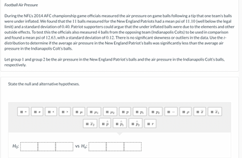
Transcribed Image Text:Football Air Pressure
During the NFL's 2014 AFC championship game officials measured the air pressure on game balls following a tip that one team's balls
were under inflated. We found that the 11 balls measured for the New England Patriots had a mean psi of 11.10 (well below the legal
limit) and a standard deviation of 0.40. Patriot supporters could argue that the under inflated balls were due to the elements and other
outside effects. To test this the officials also measured 4 balls from the opposing team (Indianapolis Colts) to be used in comparison
and found a mean psi of 12.63, with a standard deviation of 0.12. There is no significant skewness or outliers in the data. Use the t-
distribution to determine if the average air pressure in the New England Patriot's balls was significantly less than the average air
pressure in the Indianapolis Colt's balls.
Let group 1 and group 2 be the air pressure in the New England Patriot's balls and the air pressure in the Indianapolis Colt's balls,
respectively.
State the null and alternative hypotheses.
Ho:
=
H
<
V
Η μ
μ1
: x2
vs Ha:
^
:: p
μ2
:: p
^
:: P1
:: P1
^
:: P₂
:: P2
r
I
:: p
x
X1

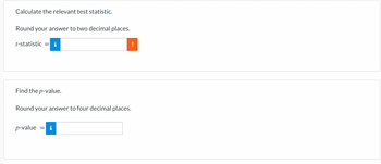
Transcribed Image Text:Calculate the relevant test statistic.
Round your answer to two decimal places.
t-statistic =
Find the p-value.
Round your answer to four decimal places.
p-value
=
IN
Expert Solution
This question has been solved!
Explore an expertly crafted, step-by-step solution for a thorough understanding of key concepts.
This is a popular solution
Trending nowThis is a popular solution!
Step by stepSolved in 2 steps with 2 images

Knowledge Booster
Similar questions
- Dr. Shoals predicts that people who walk a mile in moderately high heels will have less back pain than when they walk in very high heels. 27 participants walk in 4-inch heels and then 2.5-inch heels. He calculates the standard deviation of the difference scores and finds sD = 3.37. The mean back pain when walking in 4-inch heels is 6.75, and when walking in 2.5-inch heels, it is 3.25. What is the t statistic for this experimentarrow_forwardYoko, who turns eighty years old this year, has just learned about blood pressure problems in the elderly and is interested in how her blood pressure compares to those of her peers. She has uncovered an article in a scientific journal that reports that the mean systolic blood pressure measurement for women over seventy-five is 133.9 mmHg, with a standard deviation of 5.9 mmHg. Assume that the article reported correct information. Complete the following statements about the distribution of systolic blood pressure measurements for women over seventy-five. (a) According to Chebyshev's theorem, at least (Choose one) ▼ of the measurements lie between 122.1 mmHg and 145.7 mmHg. (b) According to Chebyshev's theorem, at least (Choose one) measurements lie between 116.2 mmHg and 151.6 mmHg. ▼ of the Xarrow_forwardPlease answer within 30min thanks.arrow_forward
- To compare the dry braking distances from 30 to 0 miles per hour for two makes of automobiles, a safety engineer conducts braking tests for 35 models of Make A and 35 models of Make B. The mean braking distance for Make A is 40 feet. Assume the population standard deviation is 4.9 feet. The mean braking distance for Make B is 44 feet. Assume the population standard deviation is 4.6 feet. At a = 0.10, can the engineer support the claim that the mean braking distances are different for the two makes of automobiles? Assume the samples are random and independent, and the populations are normally distributed. Complete parts (a) through (e). Click here to view page 1 of the standard normal distribution table. Click here to view page 2 of the standard normal distribution table. (a) Identify the claim and state H, and Ha. What is the claim? A. The mean braking distance is different for the two makes of automobiles. B. The mean braking distance is less for Make A automobiles than Make B…arrow_forwardTo compare the dry braking distances from 30 to 0 miles per hour for two makes of automobiles, a safety engineer conducts braking tests for 35 models of Make A and 35 models of Make B. The mean braking distance for Make A is 42 feet. Assume the population standard deviation is 4.7 feet. The mean braking distance for Make B is 45 feet. Assume the population standard deviation is 4.4 feet. At a = 0.10, can the engineer support the claim that the mean braking distances are different for the two makes of automobiles? Assume the samples are random and independent, and the populations are normally distributed. Complete parts (a) rari rz (b) Find the critical value(s) and identify the rejection region(s). The critical value(s) is/are (Round to three decimal places as needed. Use a comma to separate answers as needed.)arrow_forwardAfter the pandemic hit and people were forced to spend more time indoors, there have been a suspicion among health professionals. that people are eating more and thus gaining weight. In 2018, the average weight of 192 pounds, and health experts want to know if that average weight of the American male has gone up during this pandemic. d. A sample of 50 American males yeilded a sample average weight of 195 pounds and a sample standard deviation of 14.5 pounds. What is your conclusion at the 5% level of significance? (be sure to state your conclusion in the context of this problem) e. Would your conclusion change if the level of significance were changed to 1%? Briefly explain.arrow_forward
- Records indicate that the mean weight of mature rainbow trout in Eagle Creek is 1.75 kg with a standard deviation of 0.33 kg. After years of marked oxygen depletion from pollutants in the creek, a biologist wants to see if the standard deviation, o, of weights has changed. The biologist measures the weights of 20 randomly chosen mature rainbow trout from the creek and finds that the sample standard deviation is 0.38 kg. Assume the current weights of mature rainbow trout in the creek follow a normal distribution. Does the biologist have sufficient evidence to conclude that the population standard deviation, o, differs from 0.33 kg? To answer, complete the parts below to perform a hypothesis test. Use the 0.10 level of significance.arrow_forwardAn engineer designed a valve that will regulate water pressure on an automobile engine. The engineer designed the valve such that it would produce a mean pressure of 7.1 pounds/square inch. It is believed that the valve performs above the specifications. The valve was tested on 24 engines and the mean pressure was 7.3 pounds/square inch with a standard deviation of 1.0 A level of significance of 0.025 will be used. Assume the population distribution is approximately normal. Make the decision to reject or fail to reject the null hypothesis. Is it reject null hypothesis or fail to reject the null hypothesis?arrow_forwardKayla Greene is a team lead for an environmental group for a certain region. She is investigating whether the population mean monthly number of kilowatt hours (kWh) used per residential customer in the region has changed from 2006 to 2017 She is concerned that changes such as more efficient lighting and the increased use of electronics and air conditioners are affecting the mean monthly number of kilowatt hours consumed per residential customer. Kayla investigates the data and assumes the population standard deviation for 2006 and 2017 using the data that were provided to her by local utility companies. Using data that was collected by her company, Kayla selects a random sample of residential customers who were active for all of 2006 and a separate sample of residential customers who were active for all of 2017. The population standard deviations and the results from the samples are provided in the accompanying table. Explain whether a hypothesis test for the difference between two…arrow_forward
- In the 1800s, German physician Carl Reinhold, took millions of axillary (i.e. armpit) temperatures from soldiers. This study established that body temperature is normally distributed and the standard normal human body temperature is 98.6°F with a standard deviation of 0.72 °F. In a recent study, American researchers obtained 5,000 axillary temperatures from a Los Angeles hospital. The mean of these temperature readings was 97.9 F. Assuming a Type I error risk of no more than 5%, did the findings support the theory that human, body temperature has decreased since the 1800s? What is the Zcrit?arrow_forwardYou collected data from a random sample of students on their impressions of the university. On a particular opinion item item, the mean for male students was 15.2 -- with a standard deviation of 3.4. The mean on that item for women was 14.4, with a standard deviation of 3.8. Calculate Cohen's d effect size. IN THE SPACE BELOW, write the effect size AND your interpretation of it.arrow_forward
arrow_back_ios
arrow_forward_ios
Recommended textbooks for you
 MATLAB: An Introduction with ApplicationsStatisticsISBN:9781119256830Author:Amos GilatPublisher:John Wiley & Sons Inc
 Probability and Statistics for Engineering and th...StatisticsISBN:9781305251809Author:Jay L. DevorePublisher:Cengage Learning
 Statistics for The Behavioral Sciences (MindTap C...StatisticsISBN:9781305504912Author:Frederick J Gravetter, Larry B. WallnauPublisher:Cengage Learning
 Elementary Statistics: Picturing the World (7th E...StatisticsISBN:9780134683416Author:Ron Larson, Betsy FarberPublisher:PEARSON
 The Basic Practice of StatisticsStatisticsISBN:9781319042578Author:David S. Moore, William I. Notz, Michael A. FlignerPublisher:W. H. Freeman
 Introduction to the Practice of StatisticsStatisticsISBN:9781319013387Author:David S. Moore, George P. McCabe, Bruce A. CraigPublisher:W. H. Freeman

MATLAB: An Introduction with Applications
Statistics
ISBN:9781119256830
Author:Amos Gilat
Publisher:John Wiley & Sons Inc

Probability and Statistics for Engineering and th...
Statistics
ISBN:9781305251809
Author:Jay L. Devore
Publisher:Cengage Learning

Statistics for The Behavioral Sciences (MindTap C...
Statistics
ISBN:9781305504912
Author:Frederick J Gravetter, Larry B. Wallnau
Publisher:Cengage Learning

Elementary Statistics: Picturing the World (7th E...
Statistics
ISBN:9780134683416
Author:Ron Larson, Betsy Farber
Publisher:PEARSON

The Basic Practice of Statistics
Statistics
ISBN:9781319042578
Author:David S. Moore, William I. Notz, Michael A. Fligner
Publisher:W. H. Freeman

Introduction to the Practice of Statistics
Statistics
ISBN:9781319013387
Author:David S. Moore, George P. McCabe, Bruce A. Craig
Publisher:W. H. Freeman