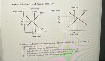
Figure: Inflationary and Recessionary Gaps Panel (a) LRAS Price level P₁ P₂ P₁ SRAS Y, Yp Real GDP AD Price level P₁ P₂ P₁ Panel (b) LRAS SRAS X Yp Y₁ Real GDP AD 10. (Figure: Inflationary and Recessionary Gaps) In Panel (b), the level of real GDP represented by Yo A) is potential output for this economy. B) C) indicates that the economy is experiencing an inflationary gap. indicates that the economy is experiencing a recessionary gap. would be associated with considerable unemployment. D)

illustrates and how it is related to the aggregate demand curve. 3. Figure 11.8 shows the aggregate expenditure curve when the price level is 110. When the price level rises to 120, the AE curve shifts vertically downwards from AE, by $1 trillion. When the price level falls to 100, the AE curve shifts vertically upwards from AE, by $1 trillion. Figure 11.8: FIGURE 11.8 Short Answer Problem 10 (a) 8 Price level (GDP deflator) Aggregate planned expendit (trillions o FIGURE 11.9 Short Answer Problem 10 (b) 130 a. Draw two new AE curves in figure 11.8 for the price levels of 100 and 120. What are the equilibrium levels of aggregate expenditures for these two price levels? Label as 'b' the equilibrium point when the price level is 100 and 'c' as price level is 120. 120 b. Use figure 11.8 to obtain three points 'a', 'b' and 'c' on the aggregate demand curve. Plot these three points on figure 11.9. Assume that the aggregate demand curve is linear and draw the AD curve on figure 11.9. Figure…

Price level (GDP price Index 2012-100) Pocential AS 130 GDP 120 110 100 90 AD 19.0 195 20.0 20.5 21.0 21.5 Real GDP (trillons of 2012 dollars) In the figure above, the economy is at an equilibrium with real GDP of $20 trillion and a price level of 110. As the economy moves toward its ultimate equilibrium, the curve shifts because O a. aggregate supply; leftward; the money wage rate rises O b. aggregate supply; rightward; the money wage rate falls O c. aggregate demand; leftward; the money wage rate rises d. potential GDP; leftward; the money wage rate falls O e. aggregate demand; rightward; the money wage rate falls

Read Eye on Booms and Busts. Explain why the NBER reported that the 2008 recession began before real GDP had fallen for two successive quarters. The NBER Committee OA. anticipated the recession was going to happen because real GDP clearly peaked in 2007 OB. based its decision on peaks in the data on real personal income, real manufacturing, wholesale and retail sales, industrial production, and employment, which all peaked between November 2007 and June 2008 OC. made an error because a recession cannot occur unless real GDP falls for two successive quarters O D. saw that the business cycle trough occurred in the second quarter of 2009, so it was obvious that the recession began in 2008

LIBR The Aggregate Expenditure or Keynesian macroeconomics model is based upon the theory that the level of GDP in the economy is determined by the level of aggregate spending. True False

The graph below shows the AD-AS diagram for the US.  How big is the inflationary gap?

4

Question 4 Which is NOT true about the natural rate of output? O It is the rate of output associated with zero unemployment. O It is also called potential GDP. O It can be referred to as full-employment GDP O It is the output associated with the LRAS curve level of output.

x ions < Price Level (average price) PE P AD, e 5.2 AD₂ 5.6 AD₁ 6.0 a AS Real Output (trillions of dollars per year) Assume aggregate demand is represented by AD1 and full employment is $5.6 trillion. The equilibrium level of income is: A) $800 billion. B) $5.2 trillion. C) $5.6 trillion. D) $6.0 trillion.

4. Assume the following model of the expenditure sector: AD=C+I+G+NX C = 420 + (4/5)YD YD=Y–TA+TR TA = (1/6)Y TRo = 100 Io = 160 Go = 180 NXo =–40 b) Assume we want to reach Y* = 2700 by changing government transfer payments (TR) instead. By how much should TR be changed?