MATLAB: An Introduction with Applications
6th Edition
ISBN: 9781119256830
Author: Amos Gilat
Publisher: John Wiley & Sons Inc
expand_more
expand_more
format_list_bulleted
Question

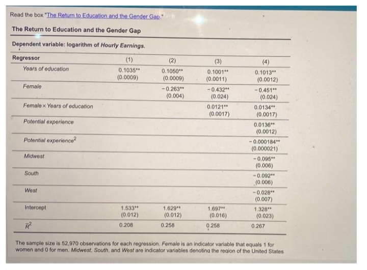
Transcribed Image Text:Read the box "The Return to Education and the Gender Gap."
The Return to Education and the Gender Gap
Dependent variable: logarithm of Hourly Earnings.
*
Regressor
Years of education
Female
Female x Years of education
Potential experience
Potential experience²
Midwest
South
West
Intercept
(1)
0.1035**
(0.0009)
1.533"
(0.012)
0.208
(2)
0.1050**
(0.0009)
-0.263**
(0.004)
1.629"
(0.012)
0.1001"
(0.0011)
0.258
-0.432**
(0.024)
0.0121"
(0.0017)
1.697**
(0.016)
(4)
0.1013**
(0.0012)
0.258
-0.451"
(0.024)
0.0134"
(0.0017)
0.0136**
(0.0012)
-0.000184**
(0.000021)
-0.095"
(0.006)
-0.092**
(0.006)
-0.028"*
(0.007)
1.328"
R²
The sample size is 52,970 observations for each regression. Female is an indicator variable that equals 1 for
women and 0 for men. Midwest, South, and West are indicator variables denoting the region of the United States
(0.023)
0.267

Transcribed Image Text:Female
Female x Years of education
Potential experience
Potential experience
Midwest
South
West
Intercept
1.533"
(0.012)
0.208
-0.263"
(0.004)
1.629"
(0.012)
-0.432**
0,024)
0.258
00121"*
(0.0017)
1.697**
(0.016)
-0.451**
(0.024)
0.258
0.0134"
(0.0017)
0.0136**
(0.0012)
-0.000184"
(0.000021)
-0.095"
(0.006)
-0.092
(0.006)
-0.028"*
(0.007)
1.328"
R²
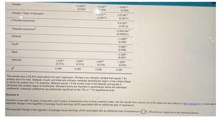
The sample size is 52,970 observations for each regression. Female is an indicator variable that equals 1 for
women and 0 for men. Midwest, South, and West are indicator variables denoting the region of the United States
in which the worker lives: For example, Midwest equals 1 if the worker lives in the Midwest and equals 0
otherwise (the omitted region is Northeast). Standard errors are reported in parentheses below the estimated
coefficients. Individual coefficients are statistically significant at the "5% or 1% significance level.
(0.023)
0.267
Scenario A
Consider a man with 18 years of education and 4 years of experience who is from a western state. Use the results from column (4) of the table and the method in Key Concept 8.1 to estimate t
expected change in the logarithm of average hourly earnings (AHE) associated with an additional year of experience.
The expected change in the logarithm of average hourly earnings (AME) associated with an additional year of experience is % (Round your response to two decimal places.)
Expert Solution
This question has been solved!
Explore an expertly crafted, step-by-step solution for a thorough understanding of key concepts.
This is a popular solution
Trending nowThis is a popular solution!
Step by stepSolved in 4 steps with 4 images

Knowledge Booster
Similar questions
- 3. у%3D-5/2хarrow_forwardTime is generally thought of as the dependant variable. O True Falsearrow_forward3-B. Write each answer with a reasonable number of figures. Find the absolute and percent relative uncertainty for each answer. 4.16 (+0.01)] X 7.068 2 (+0.000 4) = ? (a) [12.41 (0.09) (b) [3.26 ( 0.10) x 8.47 (+0.05)] - 0.18 (0.06) = ?arrow_forward
- We can use the eigenvalues and eigenvectors of ATA to express A = UΣVT as the multi- plication of three matrices U, Σ and V. The matrix Σ = 8) is a "diagonal" matrix consisting of oi's called the singular values. The values o; are formed by the square root of the positive eigenvalues of AT A ordered in decreasing order. 01 0 0 02 = • The matrix V consists of columns vectors ; called right singular vectors of A. The vectors ;'s are eigenvectors of AT A normalised so that ||vi|| 1 with respect to the standard inner product on R³. The ordering of 7; should be the same as that for σ¿. • The matrix U consists of columns vectors u¡ called left singular vectors of A. If defined, the vectors u¡ can be extracted by the identity u¡j Av. (Note: In the next part, we will show that this identity is applicable for a more general m × n matrix). Evaluate the matrices U, Σ, and V for A and validate that A = UΣVT. = σjarrow_forwardCalculate P(eating breakfast | age 14-17 )arrow_forwardUsing excel, guess the temperature of the earth in 2050 from the data below Year temperature (°C) 1880 -0.161881…arrow_forward
- The scores of a test for an engineering class of 30 students are shown here. (Due to the nature of this problem, do not use rounded intermediate values in your calculations-including answers submitted in WebAssign.) Scores: 81, 54, 55, 56, 96, 86, 98, 61, 90, 52, 92, 76, 66, 84, 79, 70, 71, 88, 62, 74, 53, 65, 55, 78, 79, 58, 60, 72, 51,80 (a) Determine the frequency (f), midpoint (x), and xf for each range and fill in the table below. (First, organize the scores into the following ranges: 50-59, 60-69, 70-79, 80-89, and 90-99.) (b) Using the following equation, determine the mean value (x) and fill in the table below. Σ(XA) n X = (c) Calculate (x − x) for each range and fill in the table below. (d) Calculate (x - x)²f for each range and fill in the table below. Range Frequency f Midpoint x 50-59 60-69 70-79 80-89 90-99 S = Enter a number. S = (e) Using the following equation, compute the standard deviation of the class scores. Σ(x-x) ²f n - 1 Σ(x-x) ²4 n - 1 = xf 29 X X - X (x - x)²farrow_forwardhow to convert a decimal nimber to a redical? with and without calculator.arrow_forward27-1/3=arrow_forward
arrow_back_ios
SEE MORE QUESTIONS
arrow_forward_ios
Recommended textbooks for you
 MATLAB: An Introduction with ApplicationsStatisticsISBN:9781119256830Author:Amos GilatPublisher:John Wiley & Sons Inc
 Probability and Statistics for Engineering and th...StatisticsISBN:9781305251809Author:Jay L. DevorePublisher:Cengage Learning
 Statistics for The Behavioral Sciences (MindTap C...StatisticsISBN:9781305504912Author:Frederick J Gravetter, Larry B. WallnauPublisher:Cengage Learning
 Elementary Statistics: Picturing the World (7th E...StatisticsISBN:9780134683416Author:Ron Larson, Betsy FarberPublisher:PEARSON
 The Basic Practice of StatisticsStatisticsISBN:9781319042578Author:David S. Moore, William I. Notz, Michael A. FlignerPublisher:W. H. Freeman
 Introduction to the Practice of StatisticsStatisticsISBN:9781319013387Author:David S. Moore, George P. McCabe, Bruce A. CraigPublisher:W. H. Freeman

MATLAB: An Introduction with Applications
Statistics
ISBN:9781119256830
Author:Amos Gilat
Publisher:John Wiley & Sons Inc

Probability and Statistics for Engineering and th...
Statistics
ISBN:9781305251809
Author:Jay L. Devore
Publisher:Cengage Learning

Statistics for The Behavioral Sciences (MindTap C...
Statistics
ISBN:9781305504912
Author:Frederick J Gravetter, Larry B. Wallnau
Publisher:Cengage Learning

Elementary Statistics: Picturing the World (7th E...
Statistics
ISBN:9780134683416
Author:Ron Larson, Betsy Farber
Publisher:PEARSON

The Basic Practice of Statistics
Statistics
ISBN:9781319042578
Author:David S. Moore, William I. Notz, Michael A. Fligner
Publisher:W. H. Freeman

Introduction to the Practice of Statistics
Statistics
ISBN:9781319013387
Author:David S. Moore, George P. McCabe, Bruce A. Craig
Publisher:W. H. Freeman