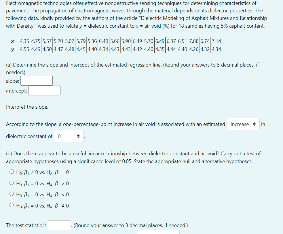
Electromagnetic technologies offer effective nondestructive sensing techniques for determining characteristics of pavement. The propagation of electromagnetic waves through the material depends on its dielectric properties. Th following data, kindly provided by the authors of the article "Dielectric Modeling of Asphalt Mixtures and Relations with Density," was used to relate y = dielectric constant to x = air void (%) for 18 samples having 5% asphalt conte x 4.35 4.75 5.57 5.20 5.07 5.79 5.36 6.40 5.66 5.90 6.49 5.70 6.49 6.37 6.51 7.88 6.74 7.14 y 4.55 4.49 4.50 4.47 4.48 4.45 4.40 4.34 4.43 4.43 4.42 4.40 4.35|4.44 4.40 4.26 4.32 4.34 (a) Determine the slope and intercept of the estimated regression line. (Round your answers to 5 decimal places, if needed.) slope:

The article "The Undrained Strength of Some Thawed Permafrost Soils" contained the accompanying data on the following. y shear strength of sandy soil (kPa) x₂-depth (m) x₂ water content (%) The predicted values and residuals were computed using the estimated regression equation 9-145.41-14.24x, +12.70x₂ +0.079x,-0.236 +0.441x where x₂-x₂²x₂-x₂², and x ₁2 Y 14.7 *2 9.1 31.6 48.0 36.5 27.1 25.6 36.7 25.8 10.0 6.0 39.2 16.0 7.0 39.3 16.8 7.0 38.4 20.7 7.4 34.0 38.8 8.3 33.7 16.9 6.4 28.0 27.0 8.1 33.0 16.0 4.6 26.4 24.9 9.8 37.9 7.3 2.8 34.5 12.8 1.9 36.3 Predicted y Residual 23.83 47.07 26.46 10.77 14.57 16.88 23.38 25.07 16.23 24.31 15.06 28.64 15.08 8.15 -9.13 0.93 -0.86 -0.77 1.43 -0.08 -2.68 13.73 0.67 2.69 0.94 -3.74 -7.78 4.65 (a) Use the given information to calculate SSResid, SSTO, and SSRegr. (Round your answers to four decimal places.) SSTO- 1x |x SSResid- SSRegr - Ix (b) Calculate R² for this regression model. (Round your answer to three decimal places.) R²-X How would you…

Solids (grams) obtained from a material as y, with respect to drying time (Hours) as x. Ten experiments were carried out to obtain the following observations: Table on the picture (a) Create a scatter diagram for the data. (b) Estimated regression model according to the data conditions. (c) Calculate Model Accuracy (R²) and Relationship Between Variables (r²)

Water is poured into a large, cone-shaped cistern. The volume of water, measured in cm, is reported at Which of the following would linearize the data for volume and time? different time intervals, measured in seconds. The scatterplot of volume versus time showed a curved Seconds, cm3 O In(Seconds), cm3 Seconds, In(cm') pattern. O In(Seconds), In(cm³)